Trading and investing performance: year eight

 Eight years! Wow. 

In late 2013 I walked out of an office for the last time where I had been working for AHL, a large systematic futures trading fund. A few months later, in April 2014, I had my own very small systematic futures trading account, and I started doing these performance reviews. And this is my eighth review. Double wow! 

As usual these cover the UK tax year, in this case from April 6th 2021 to April 5th 2022.

TLDR:

Great futures trading, no thanks to 'Black Friday', mostly thanks to the energy crisis. Outperformed AHL, but a little short of the wider index. Poor stock selection and country allocation; better in bonds; good asset allocation. Net-net: 8.2% vs my benchmark +3.8%

Overview of my world

I promised last year I would simplify things, and I have. My investments fall into the following categories:

Investing:

• 1 UK stocks
• 2 Various stock ETFs
• 3 Various bond ETFs
• 4 A small amount of uninvested cash

Trading:

• 5 Futures contracts traded by my fully automated trading strategy
• 6 Cash as trading capital for the above, of which usually around a third is required for initial margin

Excluded from this analysis is:

• My house
• A cash buffer I keep to cover living expenses

I benchmark my investments in the following way:

• A: UK single stocks 
• Benchmarked against ISF, a cheap FTSE 100 ETF (FTSE 350 is probably a better benchmark but these ETFs tend to be more expensive).
• B: Long only stocks investments: All stock ETFs and UK stocks
• Benchmarked against a cheap global equity fund (VEVE)
• C: Long only bond investments: All bond ETFs
• Benchmarked against a cheap global bond fund (AGGG)
• D: Long only investments: All UK stocks, bond ETFs and stock ETFs
• Benchmarked against a cheap 80:20 fund. 
• E: Futures trading: Return from the futures contracts traded by my fully automated system. The denominator of performance here is the notional capital at risk in my account (usually close to, but not exactly the same as the account value).
• Benchmarks are a similar fund run by my ex employers AHL, and the SG CTA index, adjusted for volatility.
• F: Everything: Long only investments, plus futures hedge, plus futures trading. I include the value of any cash included in my trading or investment accounts, since if I wasn't trading I could invest this. 
• For the benchmark I use a cheap 60:40 fund.

If you prefer maths, then the relationship to the first set of categories is:

A = 1

B = 1 + 2 

C = 3

D = B + C = 1 + 2  + 3

E = 5 + 6

F = D + 4 + E = 1 + 2 + 3 + 4  +5 + 6

If you've been following me for a while you can see that I've opted to split out my equities and bonds performance; something I haven't done before. I've also moved stuff around a bit - the 'risk' section is now under the relevant performance category, and there are some more detailed figures on costs and turnover.

Performance contribution

The figures shown are the contribution of each category to my total investment performance:

1) UK equities 1.8%

2) Stock ETFs 2.6%

3) Long only bonds 0.07%

5) Futures trading 3.7%

4 & 6) Cash 0.0%

F) Total +8.2%

Here is another way of putting it:

Long only MTM (mark to market): 1.2%

Stock and ETF dividends: 3.2%

Futures: 3.7%

Now for the same figures as 'internal rates of return', which are effectively for the 'capital' employed in each area. I use the Excel function XIRR. You can't add these up, but they are comparable and account for flows between categories. Benchmarks are also shown.

A) UK equities +9.8% Benchmark +16.6%

B) Long only stocks +6.1%   Benchmark +12%

C) Long only bonds 1.5%  Benchmark -3.0%

D) Long only investments 5.9% Benchmark +7.9%

E) Systematic futures trading  27.0% Benchmarks -4.9% +32.3% (vol matched)

F) Everything +8.2% Benchmark+3.8%

I have colour coded these to give an indication of where the good, bad and unsure are.

UK equities

This portfolio is traded using a system which I've explained before (value bias, with trailing stop of 30%), but which is not automated. Instead I have the stocks set up in a spreadsheet, with alerts reminding me when stop losses occur. If I sell then I download some data to pick the best value share.

The current portfolio looks like this:

Hammerson PLC (LSE:HMSO) 0.21%

Babcock International Group PLC (LSE:BAB) 2.45%

Greencoat UK Wind (LSE:UKW) 2.60%

Imperial Brands PLC (LSE:IMB) 3.17%

Johnson Matthey PLC (LSE:JMAT) 3.24%

Morgan Advanced Materials PLC (LSE:MGAM) 3.47%

Castings PLC (LSE:CGS) 3.50%

Barratt Developments PLC (LSE:BDEV) 3.53%

Phoenix Group Holdings PLC (LSE:PHNX) 3.64%

Lloyds Banking Group PLC (LSE:LLOY) 3.75%

BT Group PLC (LSE:BT.A) 3.82%

TP ICAP GROUP PLC (LSE:TCAP) 3.96%

Centamin PLC (LSE:CEY) 4.05%

Renewables Infrastructure Grp (LSE:TRIG) 4.24%

Greencore Group PLC 4.33%

Redde Northgate PLC (LSE:REDD) 4.39%

Aviva PLC (LSE:AV.) 4.46%

Rathbones Group Plc 4.49%

Central Asia Metals PLC (LSE:CAML) 4.58%

Morgan Sindall Group PLC (LSE:MGNS) 4.89%

Centrica PLC (LSE:CNA) 5.30%

Direct Line Insurance Group PLC (LSE:DLG) 5.87%

Investec PLC (LSE:INVP) 16.05%

Most of these were bought 'normally', but I bought a double dose of Investec last year as it was a screaming buy at a time when nothing else passed my filters (this was a good decision - see below). All are above their stops except Hammerson, which was the first share I bought coming out of the 2020 COVID market pandemic: too early as it turns out. It completely cratered before I could activate the stop and now I keep it as an out of the money call option on UK property or sentimental reminder of the importance of stops - take your pick.

Here is the performance of every share I held over the year. Percentages are taken from the start of year price, or from when I bought it during the year:

                                         MTM % Divi % TR %

Investec PLC (LSE:INVP)                         138.2% 8.3% 146.5% HELD LEGACY

Morrisons (LSE:MRW)                         62.7% 2.8% 65.5% SOLD LEGACY

Morgan Sindall Group PLC (LSE:MGNS)         33.5% 4.0% 37.4% HELD LEGACY

Babcock International Group PLC (LSE:BAB) 36.5% 0.0% 36.5% HELD LEGACY

Greencoat UK Wind (LSE:UKW)                 20.2% 5.5% 25.7% HELD LEGACY

Rathbones Group Plc                         19.6% 4.2% 23.8% HELD LEGACY

Imperial Brands PLC (LSE:IMB)                 11.5% 9.3% 20.8% HELD LEGACY

BT Group PLC (LSE:BT.A)                         17.8% 1.5% 19.2% HELD LEGACY

Aviva PLC (LSE:AV.)                         7.5% 5.2% 12.7% HELD LEGACY

Lloyds Banking Group PLC (LSE:LLOY)         8.1% 2.9% 11.0% HELD LEGACY

Senior (LSE:SNR)                         10.5% 0.0% 10.5% SOLD LEGACY

Marks And Spencer Group Plc (LSE:MKS)          8.9% 0.0% 8.9% SOLD LEGACY

Central Asia Metals PLC (LSE:CAML)          8.8% 0.0% 8.8% HELD BOUGHT

Redde Northgate PLC (LSE:REDD)                  4.3% 1.5% 5.7% HELD BOUGHT

Johnson Matthey PLC (LSE:JMAT)                  1.1% 0.0% 1.1% HELD BOUGHT

Renewables Infrastructure Grp (LSE:TRIG) -0.5% 1.2% 0.8% HELD BOUGHT

Phoenix Group Holdings PLC (LSE:PHNX)          0.6% 0.0% 0.6% HELD BOUGHT

Centrica PLC (LSE:CNA)                          0.0% 0.0% 0.0% HELD LEGACY

Hammerson PLC (LSE:HMSO)                 -2.5% 1.2% -1.3% HELD LEGACY

Morgan Advanced Materials PLC (LSE:MGAM) -3.5% 2.1% -1.4% HELD LEGACY

Centamin PLC (LSE:CEY)                         -3.9% 0.0% -3.9% HELD BOUGHT

TP ICAP GROUP PLC (LSE:TCAP)                 -6.8% 0.0% -6.8% HELD BOUGHT

Direct Line Insurance Group PLC (LSE:DLG) -14.3% 4.5% -9.8% HELD LEGACY

Royal Mail Plc (LSE:RMG)                 -13.5% 2.1% -11.5% SOLD LEGACY

Synthomer Plc (LSE:SYNT)                 -16.4% 3.7% -12.7% SOLD LEGACY

Barratt Developments PLC (LSE:BDEV)         -12.8% 0.0% -12.8% HELD BOUGHT

Castings PLC (LSE:CGS)                         -17.3% 1.0% -16.3% HELD BOUGHT

Greencore Group PLC                         -18.2% 0.0% -18.2% HELD LEGACY

Crest Nicholson Holdings Plc (LSE:CRST)         -21.0% 1.0% -20.0% SOLD LEGACY

Micro Focus International Plc (LSE:MCRO) -27.6% 3.2% -24.5% SOLD LEGACY

Vesuvius Plc (LSE:VSVS)                         -29.0% 3.8% -25.2% SOLD LEGACY

Currys Plc (LSE:DC.)                         -28.4% 2.8% -25.6% SOLD LEGACY

ITV PLC (LSE:ITV)                         -31.3% 0.0% -31.3% SOLD LEGACY

Go-Ahead group (LSE:GOOG)                 -34.5% 0.0% -34.5% SOLD LEGACY

Let me explain the columns: MTM is mark to market (the % price change since I bought it, or the start of the year), Divi(dend)% is self explanatory, TR is total return - the sum of the first two columns. The next column describes the current state of this position: do I still HOLD or have I SOLD. The final column shows when I obtained the position: at the start of the year (LEGACY) or it's something I subsequently BOUGHT.

Of course there is a bias towards selling shares that have gone down, because of the effect of the stop loss. Morrisons is an obvious exception; I sold it in October because it was being taken over and I didn't want to wait for the cash to arrive - I actually got a small premium above the final takeover price so that was a nice fluke.

I did 21 trades in this portfolio last year for a turnover of around 85%; i.e. my average holding period is probably around 15 months. That is pretty much what I expect to achieve, and I've calibrated my stop loss accordingly. It's certainly quieter than the frantic trading I did in 2020, which covered two of my performance years. Commissions came in at 0.035% of the initial portfolio value, and stamp duty tax was 0.125% plus a few quid in PTM levies. 

Stamp duty is 0.5% on buys only, but some of my shares weren't eligible (not sure why and don't really want to find out). I could avoid this by trading CFDs, but the broker I mainly use for UK shares doesn't offer these, and I'm not sure I could do this within a tax protected wrapper (as I'm actively trading, I want to avoid capital gains tax or having my trades distorted by tax optimisation).I would have paid other taxes on dividends, but generally in this post I ignore taxes.

I don't record slippage data here, but as I'm only trading FTSE 350 stocks it won't be too bad. There were other custody charges but I will account for those later since in most of my accounts I mix UK shares and ETFs (although I've since taken steps to simplify this, so I now have a single UK shares only account).

Over the year I was a net seller of UK stocks to the tune of 6% of the starting value; this was to achieve my required regional weightings (see the next section).

This has traditionally been the best part of my portfolio on a relative basis, but all good things must come to an end, or at least pause for a while. I earned an IRR of 9.8% which would be okay except the benchmark (a UK FTSE 100 tracker, ISF) returned 16.7%. It seems to finally have been the year when the much belagaured UK market actually started to catch up.

Of that sum dividends returned 3.3% - better than the 1% of last year, but still well down from the 4.6% of the year before. Forward expectations for my current portfolio show a further improvement next year, but we shall see.

2016 - 2017 XIRR  29.2%, benchmark  22.7%

2017 - 2018 XIRR  18.3%, benchmark   2.2%

2018 - 2019 XIRR  -2.3%, benchmark   7.6%

2019 - 2020 XIRR -23.1%, benchmark -24.3%

2020 - 2021 XIRR +64.3%, benchmark +24.6%

2021 - 2022 XIRR +9.8%,  benchmark +16.7%

Mean            Me 16.0%  benchmark 8.3%

Sharpe Ratio    Me 0.54   benchmark 0.45       

Geometric mean  Me 12.9%  benchmark 6.8%

Long only Stocks

As already noted this is a new category which consists of all my stock ETFs, plus my UK shares. For consistency, although it's perhaps less meaningful, here's my current portfolio of stock ETFs:

UC07 US Dividend 0.95%

PGIT* Global Infrastructure 1.46%

HMEF EM Normal         1.58%

EQDS Europe Dividend 3.69%

VHYL Global Dividend 4.30%

IAPD Asia Dividend 5.09%

PADV Asia Dividend 7.07%

PAXG Asia Normal         8.38%

IDVY Europe Dividend 9.41%

HDLG US Dividend 12.10%

EUDV Europe Dividend 12.78%

USDV US Dividend 13.10%

SEDY EM Dividend 19.20%

(PGIT is actually a UK investment trust, but I'm treating it as a stock ETF to avoid creating a new category)

Perhaps more useful are the risk exposures by region within this sub-portfolio:

              Start of year      End      Long term   Target

Asia             12%             14%         15%       14%

EM               23%             20%         25%       28%

Europe           23%             17%         20%       18%

UK               30%             29%         25%       28%

US               12%             20%         15%       12%

Start of year and End are self explanatory, whilst Long term is the strategic allocation (see my spreadsheet). After I have snapshotted the year I rebalance the portfolio to the target level shown, taking account of tax and transfers between accounts. 

Turnover on the ETF part of the portfolio was lower as I gradually rebalance according to the rules in my second book Smart Portfolios, and it came in at 30% with commisions of 0.0078%. Again I don't capture slippage here; and I will also of course be paying a management fee on my ETFs, but I try to keep this as low as possible. Incidentally a shout out to one of my brokers, iweb, who are now showing a very clear screen with all the charges you'd pay when you buy an ETF before the trade goes through. 

For the stock portfolio as a whole then then the turnover was 47%, with commissions and taxes coming in at 0.06% (most of that being the pesky taxes on UK shares). Again there are other management charges at the account level, but as I have both stocks and bonds in many accounts (I do try and keep my tax sheltered accounts purely for stock ETFs for reasons explained in Smart Portfolios, but my non tax sheltered accounts have both bonds and stocks).

I was a net buyer of stocks during the year, as will become clear below, to the tune of 12% of the starting value of the portfolio. 

Anyway, the XIRR for this weird stock/ETF hybrid beast is 6.1%, which isn't wonderful - in fact it's significantly less than the benchmark ETF I've chosen (VEVE) which returned 12%. Dividends were 3.9%.

Since the start of 2022 I'm seeing signs that my long run bets on value and the UK, and permanent US underweight, are starting to bear some fruit, so maybe this will look better next year.

No performance history here as this is the first time I've calculated this figure.

Long only Bonds

Another new section, this time with just ETFs. Current portfolio:

SLXX UK Corporate 8.48%

EMCP EM Corporate 9.00%

FAHY US High yield 9.15%

JNKE Europe High yield 10.31%

VSL* Global High yield 15.90%

VDET EM Government 19.80%

SHYG Europe High yield 27.36%

* VSL is actually a UK investment trust, but I'm treating it as a bond ETF to avoid creating a new category

Risk:

              Start of year     End      Long term   Target

Asia             1%               3%         None        5%

EM               44%             40%         25%        27%

Europe           20%             35%         25%        24%

UK               34%              8%         25%        28%

US               2%              13%         25%        16%

Note: in previous years I've classified the 'cash like' ETF XSTR as a bond ETF. This year I've classified it as cash, which makes reporting easier and also makes more sense. The UK starting risk figure above  has been recalculated to reflect this, so won't be comparable with previous years.

Note also that I don't own any Asian bond ETFs or have a long term allocation for them as there weren't any available last time I checked: the exposure shown is a 'look through' from the global bond ETFs I own.

Turnover was high in this portfolio at 178% of the average start and end value; but it's perhaps easier to point out that I was a huge net seller of bonds this year, the portfolio reducing in size by 60% (and that does not include the effect of reclassifying XSTR) which was entirely driven by net selling, not performance. Commissions were 0.044% of average capital.

The XIRR is 1.53%, which sounds mediocre until you remember we are in the middle of a massive bond bear market, and the benchmark AGGG was down -2.97%. My weighting towards  corporate and high yield rather than government bonds helped here. Dividends - or rather coupons - added a massive 4.63%. A weird year when bonds, albeit risky ones, earned me more in dividends than stocks! Although the fact I was a big net seller makes this figure hard to calculate.

Again no performance history here as this is the first time I've calculated this figure.

Long only investments

This is basically everything except my futures trading account (although to be pendantic, the odd chunks of univested cash I have lying around in my investment accounts won't be included in this section). You already know what is currently in this portfolio, and the regional risk exposures, so that just leaves the macro asset class level exposure. Here it is in cash terms:

              Start of year      End      Long term   Target

Bonds            13%             5%          22%        8%

Stock            87%             95%         78%       92%

And here's risk terms:

              Start of year      End      Long term   Target

Bonds            8%              3%          10%        5%

Stock            92%             97%         90%       95%

What has been happening here is that the sell off in bonds has driven the required allocation lower over the year. Now the needle is starting to move back - mainly due to poorer equity returns - so I'm gradually rebuilding my bond exposure although it's still only going to be half the long term target even after my current bout of rebalancing (which will take me to target).

It seems a bit weird to talk about winners and losers in the context of ETFs, but in the interests of transparancy here are the simple (not XIRR) returns for everything I held during the year in both stock and bond ETFs:

        MTM % Divi % TR %

HDLG Equity US Dividend 16.6% 3.6% 20.1%

USDV Equity US Dividend 16.0% 3.0% 19.0%

VSL* Bond Global High yield 5.4% 11.8% 17.2%

VHYL Equity Global Dividend 14.4% 0.6% 15.0%

PGIT* Equity Global Infrastructure 10.1% 4.4% 14.6%

EQDS Equity Europe Dividend 9.0% 4.8% 13.7%

UC07 Equity US Dividend 10.1% 1.8% 11.9%

JNKE Bond Europe High yield 7.1% 2.8% 9.9%

PAXG Equity Asia Normal         5.0% 3.6% 8.6%

IAPD Equity Asia Dividend -1.3% 5.2% 3.9%

SEMB Bond EM Government 1.4% 0.7% 2.1%

ISXF Bond UK High yield 0.3% 0.0% 0.3%

EMCP Bond EM Corporate -0.8% 0.4% -0.4%

PADV Equity Asia Dividend -5.8% 5.0% -0.8%

FAHY Bond US High yield -4.9% 3.5% -1.5%

SEDY Equity EM Dividend -9.5% 7.8% -1.6%

SHYG Bond Europe High yield -3.5% 1.7% -1.9%

EUDV Equity Europe Dividend -4.9% 2.5% -2.4%

VDET Bond EM Government -9.9% 6.2% -3.7%

IDVY Equity Europe Dividend -9.2% 3.9% -5.3%

HMEF Equity EM Normal         -10.3% 2.0% -8.3%

SLXX Bond UK Corporate -11.0% 1.5% -9.6%

* investment trusts, classified as ETFs

For the sake of completeness, the turnover was 58.7% on this aggregate portfolio and commissions plus taxes were 0.09%. 

You already know it was stocks good (but relatively bad), bonds bad (but relatively good), so how do we end up overall? Pretty good actually, the XIRR on all my long only investments was 5.9% which compares well to my usual benchmark, Vanguard 60:40 which returned 3.8%. However, mostly that is because my average equities allocation of around 92% cash was much higher, and equities outperformed bonds. Exactly 4% of that return was dividends.

Let's have a quick look at some history before discussing the benchmark.

2016 - 2017 XIRR  22.3%, benchmark   17.7%

2017 - 2018 XIRR   1.3%, benchmark   1.3%

2018 - 2019 XIRR   4.0%, benchmark   7.2%

2019 - 2020 XIRR -17.5%, benchmark -10.5%

2020 - 2021 XIRR +34.8%, benchmark +21.5%

2021 - 2022 XIRR  +5.9%, benchmark  +3.8%

Std. dev        Me 18.1%  benchmark 11.6%

I have said this before but it might seem a bit weird to have a 60:40 benchmark, when my long run cash allocation is closer to 80:20. The reason I have done this is because on my overall portfolio including futures trading I expect to hit vol closer to 60:40 due to diversification effects (despite my futures trading being run at 25% vol) - as you will see later, this is broadly correct. And I didn't want to use a different benchmark, because I was lazy. And indeed, the standard deviation differences above clearly show that I am running at a higher vol than 60:40

Normally changing benchmarks is cheating, but in this case it will actually make me look worse, so I hope you will allow it. So here are the restated figures again for Vanguard 80:20 as a benchmark:

2015 - 2016 XIRR   6.1%, benchmark    0.1%

2016 - 2017 XIRR  22.3%, benchmark  25.0%

2017 - 2018 XIRR   1.3%, benchmark   2.9%

2018 - 2019 XIRR   4.0%, benchmark   9.3%

2019 - 2020 XIRR -17.5%, benchmark -10.7%

2020 - 2021 XIRR +34.8%, benchmark +32.6%

2021 - 2022 XIRR  +5.9%, benchmark  +7.9%

Std. dev        Me 18.1%  benchmark 15.6%

Mean            Me 8.5%   benchmark 11.1%

Sharpe Ratio    Me 0.47   benchmark 0.72       

Geometric mean  Me 7.2%  benchmark  10.2%

The risk here still isn't spot on, but it's closer and since 80:20 is my long term target I think this new benchmark makes sense. On this revised basis then I underperformed this year, with 5.9% worse than the Vanguard 80:20 benchmark of 7.9%. This was despite my tactical weightings looking more like 90:10; but as we already know the 90% I put in stocks didn't do so well versus the benchmark. In fact a 90:10 Vanguard would have earned around 9.2%, so clearly my intra asset allocation was a bit rubbish especially in stocks.

Futures trading 

So far it's not going well, but don't worry futures will save the day :-)

Here are some statistics (all as a percentage of initial capital at the start of the year):

MTM: 24.7%

Interest: -0.07%

Fees: -0.09%

Commissions: -0.58%

Margin held, FX gain/loss: 3.1%

Net futures trading: +27.0%

Let's start with the long view:

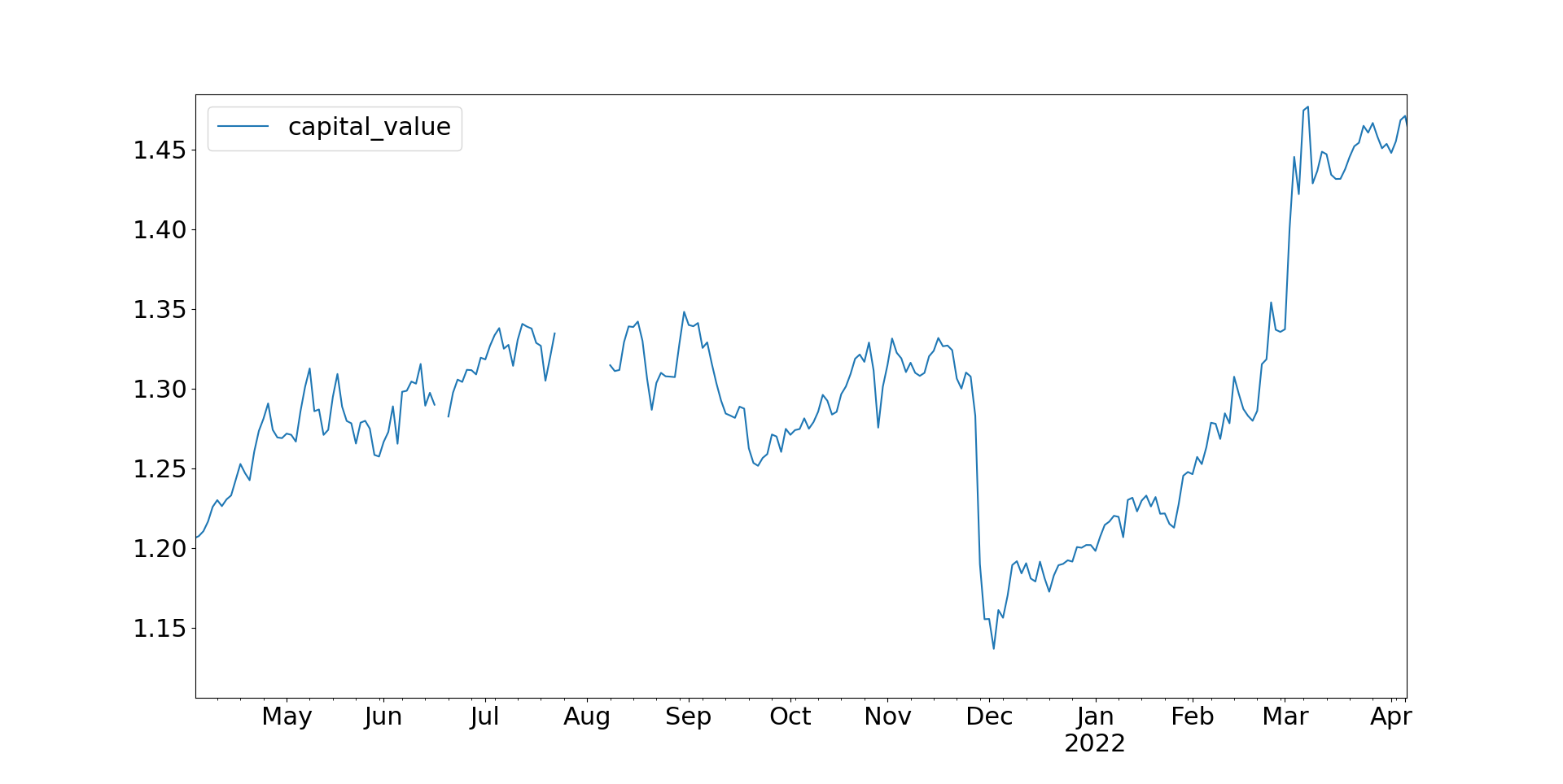
And what about last year?

Basically I had a fairly jumpy few months where I made a small net gain, then 'Black Friday', a few days in November when I lost bigly, and then of course the acceleration of the last few months. This run up ended on March 9th when there was a modest loss resulting in my risk being cut and many positions being closed. Since then I'm pretty flat.

Which markets did I make profits in?

    codes   pandl

0    Bond  -5.0

1  Metals  -2.0

2  Sector  -0.3

3     Vol   0.6

4      FX   0.9

5  Equity   1.0

6     Ags   5.1

7  OilGas  21.7

These don't add up to the total p&l for reasons I haven't got time to check now, but the general pattern is clear. This really was the year of the energy markets, with a small contribution from the Agricultural markets offset by poor performance in bonds where I struggled to deal with the bear market. This is borne out by the p&l by market list:

           codes  pandl
0           PLAT   -2.7
1            AEX   -2.5
2           BUND   -1.4
3        LEANHOG   -1.3

<SNIP>

67           OAT    1.0
68         SP400    1.2
69           VIX    1.5
70   SP500_micro    1.6
71  NASDAQ_micro    1.6
72   GAS_US_mini    1.6
73           JPY    1.9
74           SMI    2.2
75       SOYBEAN    2.8
76          CORN    2.8
77    BRENT-LAST    4.1
78  CRUDE_W_mini    4.9
79       HEATOIL    5.1
80     GASOILINE    5.7

How about costs? Total slippage was a rather hefty 2.4%, which meant I paid around 3% in total costs. This is more than I normally pay (my backtest says 1%), but I have made quite a few changes to my models this year. My new dynamic trading strategy includes costs in it's optimisation, and I've become more systematic in excluding markets that are too price to trade, so I'm comfortable this will be back under control next year.

My slippage would have been higher but I earned about 0.5% using my simple execution algo which reduced it. 

Well 27% certainly shoots the light out in absolute terms, and beats the pants off the long only benchmarks, but what about on a relative basis?

As I've done in previous years I compare this to two benchmarks, 'Bench2' the SGA CTA index, and a 'Bench1' a fund run by AHL, my ex employers. The former has daily data, but for the latter I have monthly data only, this the figures are April to March. Both benchmarks are normalised so they have the same standard deviation. I redo this normalisation every year, so the figures here won't be exactly comparable to previous years.

On this basis I returned 27% versus 38.3% for SG CTA and a loss of -4.9% for AHL. It's clearly been an excellent year for trend following, especially in the last few months; the underperformance of AHL is somewhat puzzling but they had a pretty poor January which meant that a good March didn't really get them back in the game.

My historic figures here are only for futures trading (including FX margin mark to market) - remember I used to have an equity hedge component as well. 

     My futures Bench1 Bench2

2014 – 2015 58.2% 65.9% 50.7%

2015 – 2016 23.2% -8.2% -1.6%

2016 – 2017    -14.0% -5.8%  -25.5%

2017 – 2018     -3.7%  7.0% -4.4%

2018 – 2019  5.2%  7.6%  0.8%

2019 – 2020 39.7% 21.3%  9.3%

2020 – 2021  0.4%  0.7% 12.7%

2021 – 2022 27.0% -4.9% 38.3%

Correlation      1.0     0.73    0.80

Mean         17.0% 10.5% 10.0%

Sharpe ratio 0.70  0.43  0.41

Geometric mean 14.8%  8.5%  7.7%

Of course I don't charge fees so perhaps the comparison is slightly unfair, but I'm still pretty happy with that. On a long run basis I'm outperforming both Bench1 (which did very well prior to this year) and Bench2 (which has done particularly well in the last couple of years). 

It's worth noting that my daily and monthly Sharpe Ratios are better than those shown above; this is characteristic of positive skewed assets.

Everything

Well all that remains is to add up the futures and long only performance, and see what the aggregate scorecard is. The denominator here will be the total value of all the securities and investable cash I have, including both cash for futures margin and any temporarily univested cash in other accounts. I do exclude some cash I hold as a buffer, since that can't be invested. 

The bottom line is 8.2% vs the Vanguard 60:40 benchmark of +3.8%. Dividends were 3.2% (less than the 4% before since the capital base is larger, including the dividend cash). Here's the history:

2015 - 2016 XIRR 14.4%, benchmark   0.1%

2016 - 2017 XIRR 18.2%, benchmark  19.3%

2017 - 2018 XIRR  0.6%, benchmark   1.3%

2018 - 2019 XIRR  4.4%, benchmark   7.2%

2019 - 2020 XIRR -6.6%, benchmark -10.5%

2020 - 2021 XIRR 27.9%, benchmark  21.0%

2021 - 2022 XIRR  8.2%, benchmark   3.8%

Std. dev        Me 11.7%  benchmark 10.9%

Mean            Me 9.1%   benchmark 5.9%

Sharpe Ratio    Me 0.78   benchmark 0.54       

Geometric mean  Me 8.6%  benchmark  5.4%

Note: My historic figures include the 'equity hedge' part of my portfolio which I used to have prior to this year. 

As you can see the standard deviations above are fairly close, so it seems appropriate to continue using Vanguard 60:40 as the benchmark for this part of my portfolio. The correlation - with only six observations - is 0.96. I have had three years of underperformance, followed by three years of outperformance. I'm ahead, but probably not enough to be statistically significant. Of course the latter three years span the whole COVID crisis plus Ukraine; I don't know if that is important.

Summary

It's worth briefly reviewing my plans from last year:

 I've brought some more rigour to my methodology (in the form of the model portfolio) and also done some cleaning and tidying to simplify things (removing the equity hedge).

 UK stockpicking has obviously done well, but I have no interest in substantially increasing the size of my book here, that's now up to 25 names and is also a fraction over it's tactical target allocation. 

There are 24 names listed above, although I just bought another post the end of year so that's going well. The allocation has been fairly constant.

I'm happy with my new model portfolio based approach to managing my ETF exposure; now much more formally in line with the sort of thing outlined in Smart Portfolios, and only a few minutes of work every month to keep updated. 

I'm currently in the middle of a massive refactoring of my pysystemtrade research code; once completed I hope to research and implement some new futures trading systems. Watch this space!

I certainly did that.

For this year, as I've already mentioned, I am doing some more cleaning up by making one account a pure UK stock picking account. On the futures side I'm hoping to implement some of the new trading strategies I have been researching as part of my new book, which I'm going to go back to writing once I press 'pubish'.

Is 60:40 a dead parrot? Or just resting?

 Very brief blog post this month; I'm deep into book writing mode at the moment. Chanelling Clif Assness, I'm just going to present a few charts and lead you to draw your own conclusions.

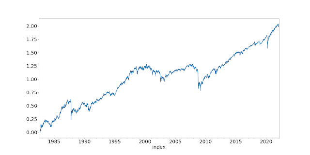
Excess / futures returns from portfolio of 60% S&P 500, 40% US Ten year treasuries (Authors own data)

Jorda et al “The rate of return on everything” QJE 2019

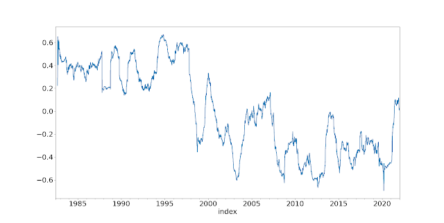
One year rolling correlation of S&P 500 and US 10 year bond daily % returns (Source; Authors own data)

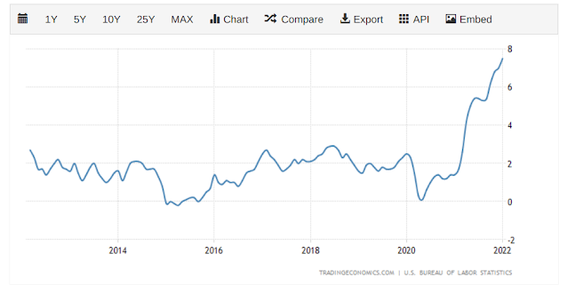
US inflation rate https://tradingeconomics.com/

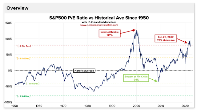
Source: https://www.currentmarketvaluation.com/

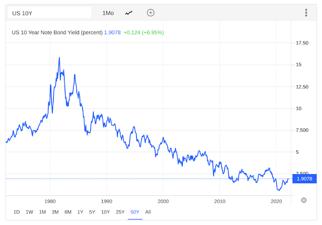
US 10 year interes rates. Source: tradingeconomics.com

And finally, for those who didn't get the Monty Python reference:

Footnote: The computing language, python, in which my trading system is written was named after Monty Python not the snake. Hence a certain publishing company that likes putting animmals on the front of their IT reference books might consider replacing the snake with a parrot...

Exogenous risk overlay: take two

This is a short follow up post to one I did a couple of years ago, on "Exogenous risk management". This was quite an interesting post which dug into why expected risk changes for a typical diversified futures trading system. And then I introduced my risk overlay:

"Now we have a better understanding of what is driving our expected risk, it's time to introduce the risk overlay. The risk overlay calculates a risk position multiplier, which is between 0 and 1. When this multiplier is one we make no changes to the positions calculated by our system. If it was 0.5, then we'd reduce our positions by half. And so on.

So the overlay acts across the entire portfolio, reducing risk proportionally on all positions at the same time. 

The risk overlay has three components, designed to deal with the following issues:

- Expected risk that is too high

- Weird correlation shocks combined with extreme positions

- Jumpy volatility (non stationary and non Gaussian vol)

Each component calculates it's own risk multipler, and then we take the lowest (most conservative) value.

That's it. I could easily make this a lot more complicated, but I wanted to keep the overlay pretty simple. It's also easy to apply this overlay to other strategies, as long as you know your portfolio weights and can estimate a covariance matrix "

Since I wrote that post, I've radically changed the way my trading strategy is designed. This is discussed at length here. Here are some relevant highlights

"Things that worked, but I decided not to implement:

• ....
• A risk overlay (actually was in my old system, but not yet in my new system - a change I plan to make soon)
• ....

Things that worked and I did implement during 2021:

• Dynamic optimisation using minimum tracking error (here and here)
• .....
• Estimating vol using a partially mean reverting method

Basically I did a lot of stuff, but along the way I lost my risk overlay. But like I said above, I planned to reintroduce it once the dust had settled. Can you hear that noise? That's sound the sound of dust settling. Also note that I introduced a new method for estimating vol. That will be important later.

There will be some very specific references to my open source trading system pysystemtrade, but the vast majority of this post should be of general interest to most people who are interested in risk management.

Where should the risk overlay go?

This was a question that wasn't an issue before, but now I have my new fancy dynamic optimisation method, where should the risk overlay go? Should it go into the upstream methodology that calculates an optimal unrounded set of positions? Or should it go into the actual dynamic optimisation itself? Or should it go into a downstream process that runs after the dynamic optimisation?

On reflection I decided not to put the overlay into the dynamic optimisation. You can imagine how this would have worked; we would have added the risk limits as additional constraints on our optimisation, rather than just multipling every positions by some factor betwen 0 and 1. It's a nice idea, and if I was doing a full blown optimisation it would make sense. But I'm using a 'greedy algo' for my optimisation, which doesn't exhaustively search the available space. That makes it unsuitable for risk based constraints. 

I also decided not to put the overlay into a downstream process. This was for a couple of reasons. Firstly, in production trading the dynamic optimisation is done seperately from the backtest, using the actual live production database to source current positions and position constraint + trade/no-trade information. I don't really want to add yet more logic to the post backtest trade generation process. Secondly - and more seriously - having gone to a lot of effort to get the optimal integer positions, applying a multiplier to these would most probably result in a lot of rounding going on, and the resulting set of contract positions would be far from optimal.

This leaves us with an upstream process; something that will change the value of system.portfolio.get_notional_positions(instrument_code) - my optimal unrounded positions. 

What risks am I concerned about?

Rather than just do a wholesale implementation of the old risk overlay, I thought it would be worthwhile considering from scratch what risks I am concerned about, and whether the original approach is the best way to avoid them. 

1. Expected risk being just too high. In the original risk overlay, I just calculated expected risk based on estimated correlations and standard deviations.
2. The risk that volatility will jump up. Specifically, the risk that it will jump to an extreme level. This risk was dealt with in the risk overlay by recalculating the expected risk, but replacing the current standard deviation with the '99' standard deviation: where % standard deviation would be for each instrument at the 99% percentile of it's distribution.
3. The risk that vol is too low compared to historic levels. I dealt with this previously in the 'endogenous' risk management eg within the system itself not the risk overlay, by not allowing a vol estimate to go below the 5% percentile of it's historic range.
4. A shock to correlations. For example, if we have positions on that look they are hedging, but correlations change to extreme values. This risk was dealt with in the risk overlay by recalculating the expected risk with a correlation matrix of +1,-1; whatever is worse.  

Here is what I decided to go with:

1. Expected risk too high: I will use the original risk overlay method
2. Vol jump risk: I will use the original method, the '99' standard deviation.
3. Vol too low risk: I have slready modified my vol estimate, as I noted above, so that it's a blend of historic and current vol. This removes the need for a percentile vol floor.
4. Correlation shock: I replaced with the equivalent calculation, a limit on sum(abs(annualised risk % each position)). This is quicker to calculate and more intuitive, but it's the same measure. Incidentally, capping the sum of absolute forecast values weighted by instrument weights would achieve a similar result, but I didn't want to use forecasts, to allow for this method being universal across different types of trading strategy.
5. Leverage risk (new): The risk of having positions whose notional exposure is an unreasonable amount of my capital. I deal with this by using specific position limits on individual instruments. 
6. Leverage risk 2 (new): The implication of a leverage limit is that there is a minimum % annualised risk we can have for a specific instrument. I deal with this by removing instruments whose risk is too low
7. Leverage risk 3: At an aggregate level in the risk overlay I also set a limit on sum(abs(notional exposure % each position)). Basically this is a crude leverage limit. So if I have $1,000,000 in notional positions, and $100,000 in capital, this would be 10.

Hence we have the following risk control measures:

• Endogenous
• Mixed vol estimate, including both long run and short run vol
• Risk overlay
• Normal: Estimated risk limit
• Jump: Estimated risk with 99% vol
• Correlation: Sum(abs(% annualised risk each position))
• Leverage: Sum(abs(notional exposure % each position))
• Off-line 
• Specific position limits to avoid any given instrument having a notional position that is too hight
• Instrument selection to avoid instruments whose % risk is too low

Off line 

Let's being by quickly talking about the 'off-line' risk controls: specific position limits, and minimum standard deviation.

Firstly, we only select instruments to trade that have some minimum standard deviation. 

It can be shown (see my forthcoming book for proof!) that there is a lower limit on the instrument risk (s), given a maximum resulting leverage ratio (size of notional position in that instrument divided by total capital) L, instrument weight w, annualised risk target (t), and instrument diversification multiplier (IDM). Assuming the ratio of maximum forecast to average forecast is 2:

Minimum s   =  (2 × IDM × w × t) ÷ L

For example, if the instrument weight is 1%, the IDM is 2.5, the risk target is 25%, and we don't want more than 100% of our notional in a specific instrument (L=1) then the minimum standard deviation is 2 * 2.5 * 0.01 * 0.25 / 1 = 1.25%. 

That's pretty low, but it would sweep up some short duration bonds. Here's the safest instruments in my data set right now:

EURIBOR         0.287279 *
SHATZ           0.553181 *
US2             0.791563 *
EDOLLAR         0.801186 *
JGB             1.143264 *
JGB-SGX-mini    1.242098 *
US3             1.423352
BTP3            1.622906
KR3             1.682838
BOBL            2.146153
CNH-onshore     2.490476

It looks like those marked with * ought to be excluded from trading. Incidentally, the Shatz and JGB mini are already excluded on the grounds of costs. 

This will affect the main backtest, since we'll eithier remove such instruments entirely, or - more likely - mark them as 'bad markets' which means I come up with optimal positions for them, but then don't actually allow the dynamic optimisation to utilise them.

Note that it's still possible for instruments to exceed the leverage limit, but this is dealt with by the off line hard position limits. Again, from my forthcoming book:

Maximum N =  L × Capital ÷ Notional exposure per contract 

          

Suppose for example we have capital of $100,000; and a notional exposure per contract of $10,000. We don’t want a leverage ratio above 1. This implies that our maximum position limit would be 10 contracts.

We can check this is consistent with the minimum percentage risk imposed in the example above with a 1% instrument weight, IDM of 2.5, and 25% risk target. The number of contracts we would hold if volatility was 1.25% would be (again, formula from my latest book although hopefully familar):

N_i = (Forecast ÷ 10) × Capital × IDM × weight_i × t ÷ 

       (Notional exposure per contract  × s_{%, i})

 = (20 ÷ 10) × 100000 × 2.5 × 0.01 × 0.25    ÷ (10,000 ×0.0125)  

 = 10 contracts

Because the limits depend on the notional size of each contract they ought to be updated regularly. I have code that calculates them automatically, and sets them in my database. The limits are used in the dynamic optimisation; plus I have other code that ensures they aren't exceeded by blocking trades which would otherwise cause positions to increase.

Note: These limits are not included in the main backtest code, and only affect production positions. It's possible in theory to test the effect of imposing these constraints in a backtest, but we'd need to allow these to be historically scaled. This isn't impossible, but it's a lot of code to write for little benefit.

Risk overlay

Once we've decided what to measure, we need to measure it, before we decide what limits to impose.

• Normal: Estimated risk limit
• Jump: Estimated risk with 99% vol
• Correlation: Sum(abs(% annualised risk each position))
• Leverage: Sum(abs(notional exposure % each position))

In my original post I noted that a way to set these limits without getting tempted to fit them, was to set them at some percentile of the distribution of each risk measure. I'm going to use the 99% percentile - the risk overlay is designed to kick in occasionally, not every other day.

I ran my full trading system (discussed here) to generate these plots; but as noted above the positions used for these calculations were unrounded positions before dynamic optimisation.

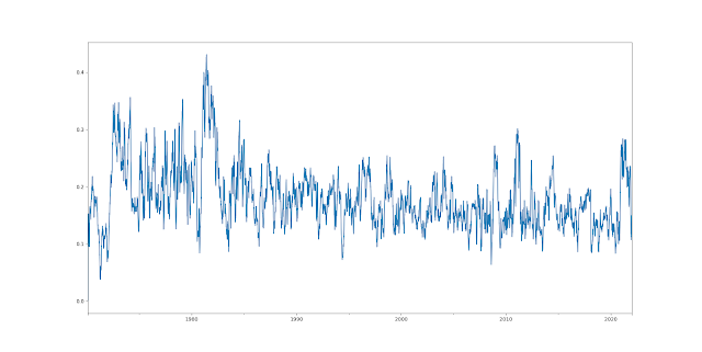
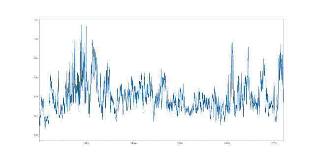
Let's start with 'normal' risk

Median: 16.9%

99% percentile: 34.9%

Notice we undershoot our risk target- 25% - and this is most likely because the IDM is capped at 2.5; so has more instruments are added we can't leverage up as much as is theoretically required.

It seems reasonable to cap this at 50% - twice the annual risk target - since we can take on positions that are twice as big than the average, if the forecast is large enough. And indeed that's what I did in the previous iteration of my risk overlay. However this would require all of our instruments to hit double forecast at the same time: unlikely! So let's stick with the 99% percentile approach and set this to 34.9/25 = 1.4 times the long run risk target. This wouldn't have been triggered in a backtest since the early 1980s.

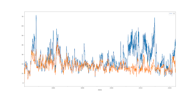
It's quite interesting to also plot the realised risk:

Here the expected risk is in orange, and the realised risk over the last 6 months is in blue. You can see that they follow each other to an extent, but we clearly realise more risk especially in the period after 2005. The median of the realised risk is much closer to target: 27%. Anyway, that's nothing to do with this post....

Now for the 'jump' risk

Median: 36.8%

99% percentile: 89.5%

This equates to a risk limit of 89.5/25 = 3.6 times normal risk. It's a bit lower than the 6 times I used before, probably reflecting a more diversified portfolio. This would have been triggered in the late 1970's and early 1980's, plus in 2011, 2014 and 2021.

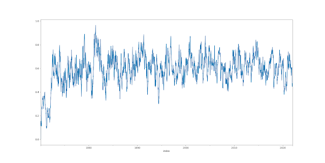
Now, correlation risk:

Median: 60.3%

99% percentile: 84.6%

This equates to a risk limit of 84.6/25 = 3.4 times normal risk. This would have been trigerred, briefly, in 2014.

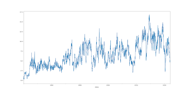
Finally, leverage:

Remember the units here aren't % annualised risk, they are a ratio to capital.

Median 6.15

99% percentile: 13.9

This is a tricky one, and if you're going to use this approach I would advise checking for yourself since the leverage will depend very much on the mixture of instruments you have. The leverage has clearly grown over time as more instruments have been added with lower risk. On the face of it, 13.9 times leverage sounds pretty flipping scary. 

But remember that the use of position limits in production, and the avoidance of instruments with very low risk, will probably mean the real leverage isn't as bad as all this. For example, the leverage I have on at this very moment with my actual production positions after dynamic optimisation is just 1.6 times.

Anyway we have to use a number, so let's be a tiny bit more conservative than 99% percentile and go for lucky 13.

Here's the limits in the configuration in case you want to change them:

risk_overlay:
  max_risk_fraction_normal_risk: 1.4
  max_risk_fraction_stdev_risk: 3.6
  max_risk_limit_sum_abs_risk: 3.4
  max_risk_leverage: 13.0

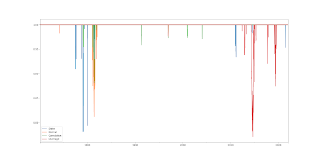
Now, for each of the risk measures I calculate the following scalar: Min(1, Limit / Risk measure). 

That will be equal to 1 most of the time, and lower than 1 if the risk measure has exceeded the limit.

We'd then take the minimum value of these four ratios. Notice that different risk ratios are kicking in at different times, as different risk measures become problematic.

The longest period the risk overlay is turned on is for about 6 months in late 2014. Mostly though it just kicks in for a few days. The minimum value is 0.77; so we'd reduced our position by almost a quarter. The overlay is on about 4% of time; this feels about right given we have four risk measures kicking in 1% of the time, so that's what we'd expect if they were uncorrelated.

Finally I multiply the unrounded positions (pre dynamic optimisation) by this risk scaler value. 

There will be additional trading costs from implementing this; if I wasn't using the dynamic optimisation that provides a buffering service, I'd probably think about smoothing the risk overlay a little bit to reduce those costs.

I won't be bothering to test the effect of running this risk overlay; it doesn't turn on enough to give meaningful results. 

Summary

That's probably it in terms of modifying my flagship system for a while - probably a good thing after quite a few changes in a relatively short time!