As those of you who follow me on the Elon Musk Daily News App will know, I received physical copies of my new book last week (exciting!). Global supply chains being what they are, you lot will have to wait until April to get your copies. Sorry.
Anyway one of the themes I touch on in the book is the truely amazing diversification that trend following strategies offer when run across multiple instruments.
I have touched on this before (although never in detail with a complete blogpost on the subect), but I thought I would present some updated results using the data set I use in the book (102 instruments), presented with some different plots to help better grasp the intuition of what's going on. This isn't a sneak preview of stuff in the book, you'll still have to buy it :-), but goes into more detail to help understand just how amazing this effect.
Incidentally I don't trade butter because it isn't liquid enough; less than 20 contracts a day. Maybe if I left it out of the fridge in hot weather....
(Code is here. These results are not exactly the same as in my latest book, as I'm using a different methodology)
Measuring diversification
The most intuitive way to measure diversification is a simple ratio: expected return for many things divided by the expected return for one thing.
But there is another way of measuring diversification through 'independent bets', which I was reminded of when I reread this 2018 article by the always excellent Cory Hoffstein, and also this article by Resolve (Adam Butler et al).
Cory's article talks about the three axis of diversification: what, how and when. That article talks a great deal about 'how': diversification across trading rules in my parlance. This blogpost and the Resolve post consider 'what': diversification across instruments. You can also consider 'when': broadly speaking, diversifying across different forecast horizons or speeds of trading rules.
The maths behind the independent bet idea is simple; if you have a portfolio of N return streams (eg trading strategies running on different instruments), scaled to the same volatility (normal for trading strategies) and they are uncorrelated, then your standard deviation will reduce by sqrt(N) versus the risk of one strategy. Assuming they have the same expected mean, your Sharpe Ratio will therefore increase by sqrt(N). If you can use leverage (like a futures trader), then you can purchase higher returns with that rise in Sharpe Ratio.
Most portfolios aren't uncorrelated, so we can bring in the idea of effective independent bets. That's just the value of N with uncorrelated assets that would give you the same reduction in standard deviation that you actually get in practice. For example, if your correlation is 0.5 with two assets equally weighted, then your SR will increase by 1.15. That is the same improvement that we would get from having 1.15^2 = 1.33 independent bets.
Similarly, if we have three assets with an average correlation of 0.5, then the SR will improve by 1.225 which is the same as having 1.5 independent bets.
A couple of wrinkles: The average correlation is a nice guide, but in the actual calculation you should use the entire correlation matrix. Also, the simple independent bets calculation assumes that all your assets are equally weighting in the zero correlation version. But in calculating the standard deviation for the uncorrelated portfolio you should use the actual weights.
For example, with identical off diagonal correlations of 0.3 and equal weights, there are 1.88 independent bets. But consider this piece of pysystemtrade code:
from sysquant.estimators.diversification_multipliers import *
corr = correlationEstimate(np.array([[1,0.5, .3], [.5,1, .1], [.3,.1,1]]), columns=['a', 'b','c'])

     a    b    c
a  1.0  0.5  0.3
b  0.5  1.0  0.1
c  0.3  0.1  1.0

corr.average_corr()
0.3

weights = portfolioWeights(dict(a=.45, b=.45, c=.1))

## independent bets
diversification_mult_single_period(corrmatrix=corr, weights=weights)**3
1.53
By allocating less to the more diversifying asset we have reduced the available diversification.
However in this post I will always optimise instrument weights to minimise the portfolio standard deviation using only the correlation matrix as an input, hence maximising the available diversification.
Now, there two ways to calculate diversification, eithier as a ratio of standard deviations (Sharpe Ratios) or as a number of independent bets. The first is to use the correlation matrix of returns, and weights, as I've already done. We can think of this as expected diversification benefit. In fact I do this already in my code - it's called the instrument diversification multiplier (IDM). So if take IDM^2 then that will be equal to the expected benefit, measured in units of independent bets.
The second way of measuring diversification is by looking at the realised Sharpe Ratio of the portfolio, and comparing that to the Sharpe Ratio for a single instrument. We can think of that as the realised diversification benefit. And if I square that ratio, I will again get the realised benefit measured in independent bets.
There is a third way, which is to measure the realised standard deviation of the portfolio having not applied any diversification multiplier. But assuming we are pretty good at predicting risk - and we are - this will be pretty similar to the IDM figure.
So in summary we can measure:
- Expected diversification ratio (equivalent to IDM)
- Expected number of independent bets (IDM^2)
- Realised diversification ratio (SR ratio)
- Realised diversification as a number of independent bets
Which markets?
There is a big problem here, which is that we're comparing the diversification of one instrument with say two instruments. But which 'one instrument'? And which two instruments? We'll get different answers if we compare a portfolio of Corn and US 10 year bonds versus a portfolio with just Eurodollar, or a portfolio of Dry milk and Crude oil, versus just US 2 year.
That isn't so much of a problem with correlations, but for Sharpe Ratio which exhibits a lot of variation across instruments, it's a big problem.
The answer, is to Monte Carlo this. For each portfolio size N that we want to test we run a bunch of different random runs. Each run involves picking a random group of N markets, allocate instrument weights, and measure the resulting portfolio IDM (expected diversification) and Sharpe Ratio. Then we take the average (median) to get the values for a given N.
Incidentally I calculated instrument weights in two ways to check the robustness of my results:
- Optimised using using correlation as an input into the optimisation, with flooring at zero and some shrinkage for stability.
- Equal weights. I have some heterogeneity in my instruments, eg a lot of equities, so this may not be appropriate.
Long only
Let's first consider a long only portfolio. This will be identical to the trend following portfolio except it uses a constant forecast (the 'asset allocating investor in my first book').
Interestingly, the average correlation of instrument returns across the entire portfolio of 102 instruments is 0.224 (effective number of independent bets, 4.3), but the correlation of subsystem returns (basically trading each instrument, sizing positions for current volatility) is just 0.09 (number of independent bets 6.3).
First of all let's look at the expected diversification, measured by IDM, with optimised weights. Just to give you a flavour of the monte carlo, the following plot shows the individual data points for each monte carlo, plus a median line. Notice the noise falls as we get more instruments; that's because the portfolios get more similar. At the limit when we're choosing 100 out of 103 instruments, the results are going to be fairly similar.

At the top end the IDM is around 4.8, which means we've got 4.8^2 = 23 independent bets.
Note: I am optimising weights in such a way that will maximise the IDM, hence the IDM's here are higher than in the book for both long only and trend following strategies.
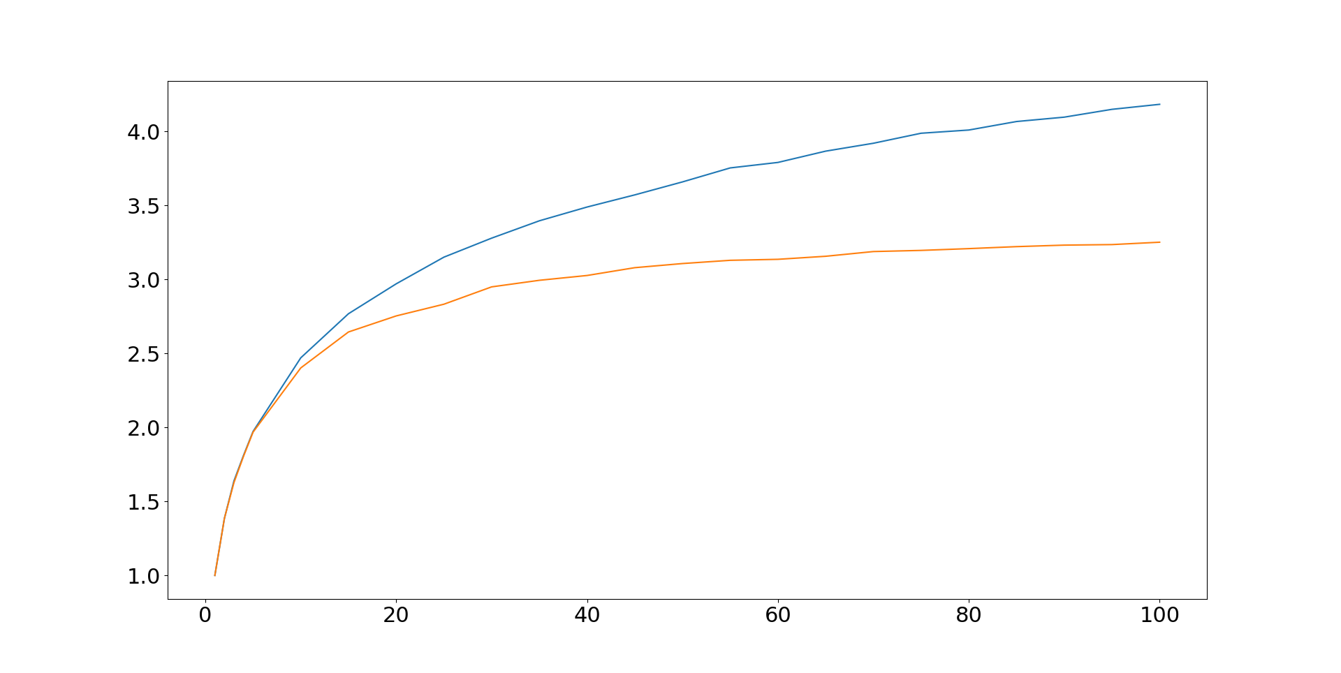
This sounds pretty amazing, but what about the Sharpe ratio, realised diversification? To get something with a comparable y-axis we need to divide the Sharpe Ratios by the median SR for a single instrument. Here is what we get:


Trend following
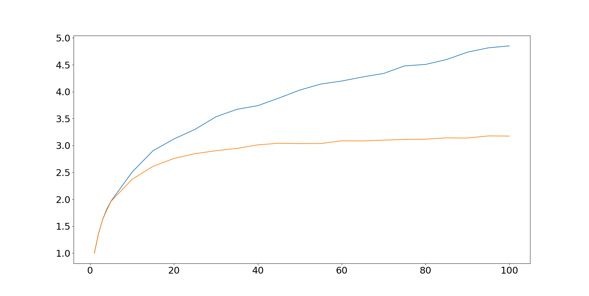
Now let's consider the same setup, but for a trend following strategy. For simplicity I just used a single trading rule, the EWMAC16,64 rule AKA the starter system from Leveraged Trading. But the results will be similar for a portfolio of such rules. First of all let's plot the IDM, for both optimised (blue) and equal weights (orange).

Another important point is that it looks like the blue line here is still going, suggesting adding even more instruments could potentially boost SR further. In contrast the long only portfolio asymptotes at around 50 instruments, with further diversification not adding anything meaningful.
Summary
Whenever I have plotted these graphs before it has always been to make the point that instrument diversification is the best kind. Adding different kinds of trading rule, or trading at different speeds, or both, will boost your performance - but not by very much. You will be lucky to get two independent bets worth of diversification from this source. In contrast, we can get realised performance equivalent to over twenty independent bets from diversifying across a trend following portfolio of 100 instruments; versus just over four in a long only setup (and it would be even lower without volatility targeting!).
Unfortunately adding instruments requires more capital or doing something smart like my own dynamic optimisation technique. Diversification is a free lunch, but you still need to get to the buffet...