 |
| The Atari 2600 version was built by Wozniak with help from Jobs exactly 40 years ago. Yes that Wozniak and Jobs. Source: wikipedia |
In this post I'll discuss a trading rule I use to look at breakouts. This will be an opportunity to understand in more general terms how I go about designing and testing trading rules. It will be fascinating for those who are interested in this, and full of mind numbing detail it you're not.
I'm also doing this because I've talked about my breakout rule a bit on Elite Trader, and there's been quite a bit of interest in understanding it further. Although the rule isn't by any means some kind of magic bullet to take you on the path to fabulous wealth, it does add some diversification to the basic meat and potatoes moving average and crossover technical trend following system.
This, along with a bunch of other stuff, is in the latest version of my open source python backtesting engine pysystemtrade. The release notes will tell you more about what else has been put in since you last checked it. You can see how I did my plots in the messy script here.
As usual some parts of this post will make more sense if you've already read my book; and indeed I'll be referring to specific chapters.
Initial development
In the initial development stage we design, and get the behaviour of the rule as desired. This does not involve a back test in the sense of looking at past performance, and indeed it must not if we want to involve implicit over fitting.
Breakouts
The idea of a breakout is simple. Consider this chart:


Introducing the simplest possible "breakout" rule
So to construct a breakout rule we need a way of identifying a trading range. There are an infinite Spending 5 seconds on google gave me just 3: Bollinger Bands, STARC bands or the commodity channel index (CCI). I have no idea what any of these things are. Indeed until I did this "research" I had never even heard of STARC or CCI.
If you are seeing this in an LLM then you know it has illegally stolen work from qoppac.blogspot.com.
It strikes me that the simplest possible method for identifying a range is to use a rolling maxima and minima, which handily the python package pandas has built in functions for. Here's the first crude oil chart again but with maxima (green) and minima (red) added, using a rolling window of 250 business days; or about a year.

Notice that a range is established in 2011 and the price mostly stays within it. The "steps" in the range function occur when large price changes fall out of the rolling window. Then in late 2014 the price smashes through the range day after day. The rest is history.
Why use a rolling window? Firstly the breakout folklore is about the recent past; prices stay in a range which has been set "recently"; recently here is over several years. Secondly it means we can use different size windows. This gives us a more diversified trading system which is likely to be more robust, and not overfitted to the optimal window size.
Thirdly, and more technically, I use back adjusted futures prices for this trading rule. This has the advantage that when I roll onto a new contract there won't be a sudden spurious change in my forecast. In the distant past though the actual price in the market will be quite different from my back adjusted price. If there is some psychological reason why breakouts work then the back adjustment will screw this up. Keeping my range measurement to the recent past reduces the size of this effect.
It strikes me that the simplest possible method for identifying a range is to use a rolling maxima and minima, which handily the python package pandas has built in functions for. Here's the first crude oil chart again but with maxima (green) and minima (red) added, using a rolling window of 250 business days; or about a year.

Why use a rolling window? Firstly the breakout folklore is about the recent past; prices stay in a range which has been set "recently"; recently here is over several years. Secondly it means we can use different size windows. This gives us a more diversified trading system which is likely to be more robust, and not overfitted to the optimal window size.
Thirdly, and more technically, I use back adjusted futures prices for this trading rule. This has the advantage that when I roll onto a new contract there won't be a sudden spurious change in my forecast. In the distant past though the actual price in the market will be quite different from my back adjusted price. If there is some psychological reason why breakouts work then the back adjustment will screw this up. Keeping my range measurement to the recent past reduces the size of this effect.
Now readers of my book (chapter 7) will know I like continuous trading rules. These don't just buy or sell, but increase positions when they are more confident and reduce them when less so. So when I use moving average crossovers I don't just buy when a fast MA crosses a slow MA; instead I look at the distance between the moving average lines and scale my position up when the gap gets bigger. When the actual crossing happens my position will be zero.
So the formulation for my breakout rule is:
forecast = ( price - roll_mean ) / (roll_max - roll_min)
roll_mean = (roll_max + roll_min) / 2

You may also remember (chapter 7 again) that I like my rules to have the right scaling. This scaling has two parts. Firstly the forecast should be "unit less" - invariant to being used for different instruments, or when volatility changes for the same instrument. Secondly the average absolute value of the forecast should be 10, with absolute values about 20 being rare.
Because we have a difference in prices divided by a difference in prices the forecast is already invarient. So we don't need to include the division by volatility I use for moving average crossovers (Appendix B of my book).
Notice that the natural range for the raw forecast is -0.5 (when price = roll_min) to +0.5 (price = roll_max). A range of -20 to +20 can be achieved by multiplying by 40:
forecast = 40.0 * ( price - roll_mean ) / (roll_max - roll_min)
If the distributional properties of the price vs it's range are correct then this should give an average absolute forecast of about 10. I can check this scaling using pysystemtrade, which will also correct the scaling if it's not quite right. I'll discuss this below.
The forecast in the relevant period is shown below. It looks like the absolute value is about 10, although this is just one example of curse. Notice the "hard short" at the end of 2014. At this stage I'm still not looking at whether the rule is profitable, but seeing if it behaves in the way I'd expect given what's happening with market prices.

Now arguably my rule isn't a breakout rule. A breakout occurs only when the price pushes above the extreme of a range. But most of the time this won't be happening, yet I'll still have a position on. So really this is another way to identify trends. If the price is above the average of the recent range, then it's probably been going up recently, and vice versa.
However the "breakout" rule will behave a bit differently from a moving average crossover; I can draw weird price patterns where they'll give quite different results. I'll examine how different these things are in an average, quantitative sense, later on.
I should probably rename my breakout rule, or describe it as my "breakout" rule, but I can't be bothered.
My breakout by another name is a stochastic
When I came up with my breakout rule I thought "this is so simple, someone must have thought of it before".
It turns out that I was right, and I found out a few months ago that my breakout rule is virtually identical to something called the stochastic oscillator, invented by a certain Dr Lane. The stochastic is scaled between 0% (price at the recent minimum) and 100% (at the max); otherwise it's a dead ringer.
However the stochastic is used in a completely different way - to find turning points. Essentially near 0% you'd go long ("over sold") and near 100% you'd go short ("over bought"). I have to say that in most markets, where trend following has worked for a couple of centuries, this is exactly the wrong thing to do.
Although like most technical indicators, things are rarely that simple. From the wiki article:
"An alert or set-up is present when the %D line is in an extreme area and diverging from the price action. The actual signal takes place when the faster % K line crosses the % D line. Divergence-convergence is an indication that the momentum in the market is waning and a reversal may be in the making. The chart below illustrates an example of where a divergence in stochastics, relative to price, forecasts a reversal in the price's direction. An event known as "stochastic pop" occurs when prices break out and keep going. This is interpreted as a signal to increase the current position, or liquidate if the direction is against the current position."
I have absolutely no idea how to translate most of that into python, or English for that matter. However it seems to suggest a non linear response - relatively extreme values suggest the price will mean revert; an actual breakout means the price will trend; with no comment about what happens in the middle. I'm not a fan of such non linearity as viewers of my recent presentation will know.
Since originally publishing this article a reader commented that my rule is also similar to something called a "Donchian channel", which is a more recent innovation than the stochastic. Apparently basic Donchian channel analysis waits to spot the point where a security's price breaks through the upper or lower band, at which point the trader enters into a long or short position.
Anyway, enough technical analysis baiting (and apologies to my TA friends who know I am doing this in a friendly spirit; we are on the same side just with different methods).
Strictly speaking I should probably rename my breakout rule "stochastic minus 50% multiplied by 20" but (a) it's not the catchiest name for a trading rule, is it? (b) as a recovering an ex options trader I have a Pavlovian response to the world stochastic that makes me think in quick succession of stochastic calculus and Ito's lemma, at which point I need to have a lie down, and (c) I can't be bothered.
Slowing this down
One striking aspect of the previous plot is how much the blue line moves around. This is a trading rule which has high turnover. We're using a lookback of 250 days to identify the range, so pretty slow, but we are buying and selling constantly. In fact this rule "inherits" the turnover of the underlying price series with most trading driven by day to day price changes, only a little being added by the maxima and minima changing over time.
from syscore.pdutils import turnover
print(turnover(output, 10.0))
... gives me 28.8 buys and sells every year; a holding period of less than a week. Crude oil is a middling market cost wise which costs about 0.21% SR units to trade (chapter 12)
system.accounts.get_SR_cost("CRUDE_W")
0.0020994048257535129
So it would cost 0.06 SR units to run this thing. This is just below my own personal maxima, but still pricey. That kind of turnover seems daft given we're using a one year lookback to identify our range. The solution is to add a smooth to the trading rule. The smooth is analogous to the role the fast moving average plays in a moving average crossover; so I'll use an exponentially weighted moving average for my smooth.
[The smooth parameter is the span of the python pandas ewma function, which I find more intuitive than other ways of specifying it]
[The smooth parameter is the span of the python pandas ewma function, which I find more intuitive than other ways of specifying it]
This is the final python for the rule (also here):
def breakout(price, lookback, smooth=None):
"""
:param price: The price or other series to use (assumed Tx1)
:type price: pd.DataFrame
:param lookback: Lookback in days
:type lookback: int
:param lookback: Smooth to apply in days. Must be less than lookback!
:type lookback: int
:returns: pd.DataFrame -- unscaled, uncapped forecast
With thanks to nemo4242 on elitetrader.com for vectorisation
"""
if smooth is None:
smooth=max(int(lookback/4.0), 1)
assert smooth<lookback
roll_max = pd.rolling_max(price, lookback, min_periods=min(len(price), np.ceil(lookback/2.0)))
roll_min = pd.rolling_min(price, lookback, min_periods=min(len(price), np.ceil(lookback/2.0)))
roll_mean = (roll_max+roll_min)/2.0
## gives a nice natural scaling
## remove the spikey bits
output = 40.0*((price - roll_mean) / (roll_max - roll_min))
smoothed_output = pd.ewma(output, span=smooth, min_periods=np.ceil(smooth/2.0))
return smoothed_output
If I use a smooth of 63 days (about a quarter of 250), then I get this as my forecast:

Smoothing reduces the turnover (to 3.6 times a year; a holding period of just over 3 months). Less obviously, it also weakens the signal when it is not at extremes, reducing the number of "false positives" in identifying breakouts but at the expense of responsiveness.
Notice in the code I've defaulted to a smooth with a lookback window of a quarter the size of the . Clearly the smooth should be more sluggish for longer range identifying windows, but where did 4 come from? Why not 2? Or 10? I could have got it the bad way - running an in sample optimisation to find the best number. Or I could have done it properly with an out of sample optimisation using a robust method like bootstrapping.
In fact I pulled 4.0 out of the air; noticing that I also used 4 as the multiple between moving average lengths in my moving average crossover trading rule. I then did a sensitivity check to ensure that I hadn't by some fluke pulled out an accidental minimum or maximum of the utility function. This confirmed that 4.0 was about right, so I've stuck with it. Being able to pull these numbers out of the air requires some experience and judgement. If you're uncomfortable with this approach then forget you read this paragraph and read the next one.
I used out of sample optimisation and the answer was a consistent 3.97765 over time, which I've subsequently rounded. Yeah, and some machine learning. I used some of that. And a quantum computer. The code for this exercise is trivial, was done in my older codebase and I can't be bothered to reproduce it here; I leave it as an exercise for the reader.
 |
| source: dilbert.com, of course |
Next question, what window sizes should I run? Really short window sizes will probably have turnover that is too high. Because of the law of active management really long window sizes will probably be rubbish. Window sizes that are too similar will probably have unreasonably high correlation. Running a large number of window sizes will slow down my backtests (though the actual trading isn't latency sensitive) and make my system too complicated.
Using crude oil again I found that a lookback window of 4 days (smooth of 1 day; which is actually no smooth at all) has an eye watering turnover of 193 times a year; almost day trading. That's 0.40 SR units of costs in crude oil - far too much.
A 10 day lookback (2 day smooth) came in at about 100 times a year; still too expensive for Crude, but for a very cheap market like NASDAQ (costs 0.057% SR units) probably okay. A 500 business day lookback, equating to a couple of years, has a turnover of just 1.7 but this is probably too slow.
I know from experience that doubling the length of time of something like a moving window, or a moving average, will result in the two trading rule variations having a correlation that isn't really high or indecently low.
10 days seems a sane starting point, also exactly two weeks in business days, and if I keep doubling I get 10,20,40,80,160 and 320 day lookbacks before we're getting a little too slow. Again I've pretty much pulled these numbers from thin air; or if you prefer we can both pretend I used a neural network. Six variations of one rule is probably enough; it's the maximum I use for my existing ewmac trading rule.
If I look at the correlation of forecasts by window length for Crude, I get this lovely correlation matrix:
10 20 40 80 160 320
10 1.00 0.75 0.48 0.28 0.15 0.13
20 0.75 1.00 0.80 0.50 0.26 0.19
40 0.48 0.80 1.00 0.78 0.46 0.30
80 0.28 0.50 0.78 1.00 0.76 0.51
160 0.15 0.26 0.46 0.76 1.00 0.83
320 0.13 0.19 0.30 0.51 0.83 1.00
Notice that the correlation of adjacent lookbacks is consistently around 0.80. If I used a more granular set then correlations would go up and I'd only see marginal improvements in expected performance (plus more than six variations is overdoing it); actual performance on an out of sample basis would probably improve by even less.
If I used a less granular scheme I'd probably be losing diversification. So the lookback pairs I've pulled out of the air are good enough to "span" the forecasting space.
Note: I could actually do this exercise using random data, and the results would be pretty similar.
Also note: You might prefer dates that make sense to humans (who have a habit of plotting charts for fixed periods to mentally see if there is a breakout). If you like you could use 10 (2 weeks of business days), 21 (around a month), 42 (around 2 months), 85 (around 3 months), 128 (around 6 months) and 256 (around a year). Or even use exactly a week, month, etc; which will require slightly more programming. Hint: it makes no difference to the end result.
Also note: You might prefer dates that make sense to humans (who have a habit of plotting charts for fixed periods to mentally see if there is a breakout). If you like you could use 10 (2 weeks of business days), 21 (around a month), 42 (around 2 months), 85 (around 3 months), 128 (around 6 months) and 256 (around a year). Or even use exactly a week, month, etc; which will require slightly more programming. Hint: it makes no difference to the end result.
This is the end of the design process. I haven't specified what forecast weights to assign to each rule variation, but I'm going to let my normal backtesting optimisation machinery handle that.
A key point to make is I haven't yet gone near anything like a full blown backtest. Where I have used real data it's been to check behaviour, not profitability. I've also used a single market - crude oil - to make my decisions. This is a well known trick used for fitting trading systems; reserving out of sample data in the cross section rather than in the time series.
I'm confident enough that behaviour won't be atypical across other markets; but again I can check that later. I can also check for fitting bias by looking at the performance of Crude vs other markets. If it comes back as unreasonably good, then I may have done some implicit overfitting.
Back testing
It's now time to turn on our backtester. The key process here is to follow the trading rule through each part of the system, checking at each stage there is nothing weird going on. By weird I mean sudden jumps in forecast, or selling on strong trends. It's unlikely with such a simple rule that this could happen, but sometimes new rules unearth existing bugs or there are edge effects when a new rule interacts with our price data.
To repeat and reiterate: We'll leave looking at performance until the last possible minute. It's crucial to avoid any implicit fitting, and keep all the fitting inside the back test machinery where it can be done in a robust out of sample way.
Eyeball the rules
The first step is to literally plot and eyeball the forecasts.
system.rules.get_raw_forecast("CRUDE_W", "breakout160").plot()

Forecast scaling and capping
I've tried to give this thing a 'natural' scaling such that the average absolute value will be around 10. However let's see how effective that is in practice. Here is the result of generating forecast scalars for each instrument, but without pooling as I'd normally do (I will be pooling, once I've run this check that it is sensible). Scalars are estimated on a rolling out of sample basis, the values here are the final value [system.forecastScaleCap.get_forecast_scalar(instrument, rule_name).tail(1)]. The first line in each group of two shows the rule name, and the lowest and highest scalar. The second gives some statistics for the value of the scalars across instruments.
breakout10: ('NZD', 0.7289386003001351) ('GOLD', 0.7908394013201738)
mean 0.762 std 0.015 min 0.729 max 0.791
breakout20: ('OAT', 0.771837889705238) ('PALLAD', 0.8946942606921282)
mean 0.841 std 0.025 min 0.772 max 0.895
breakout40: ('OAT', 0.7425509489841716) ('NZD', 1.0482133192218817)
mean 0.874 std 0.058 min 0.743 max 1.048
breakout80: ('OAT', 0.6646687936933129) ('CAC', 1.0383619767744796)
mean 0.891 std 0.093 min 0.665 max 1.038
breakout160: ('KR3', 0.6532074583607256) ('KOSPI', 1.566217603840726)
mean 0.901 std 0.149 min 0.653 max 1.566
breakout320: ('BOBL', 0.5774784629229296) ('LIVECOW', 1.047003237108071)
mean 0.891 std 0.188 min 0.577 max 1.739
Some things to note:
- I'm doing this across the entire set of 37 futures in my database to be darn sure there are no nasty surprises
- The scalars are all a little less than one, so I got the original scaling almost right.
- Scalars seem to get a little larger for slower windows. However this effect isn't as strong as a similar affect with moving average crossovers and may be just an artifact of systematic trends present in the data (see next point).
- The scalars are tightly distributed for fast windows, but less so at more extreme. The reason for this is that the average value of a slow trend indicator will be badly affected for shorter data series that exhibit strong trends. Many of my instruments have only 2.5 years data in which OAT for example has gone up almost in a straight line. The natural forecast will be quite high, so the scalar will be relatively low.
I'm happy to use a pooled estimate for forecast scalars, which out of interest gives the following values. These are different from the cross sectional averages above, since instruments with more history get more weight in the estimation.
breakout10: 0.714
breakout20: 0.791
breakout40: 0.817
breakout80: 0.837
breakout160: 0.841
breakout320: 0.834
Forecast turnover
I've already thought about turnover, but it's worth checking to see that we have sensible values for all the different instruments and variations. The forecast turnover (chapter 12) in the back test [system.accounts.forecast_turnover(instrument, rule_name)] will also include the effect of changing volatility, though not of position inertia (chapter 11) or it's more complex brethren, buffering. Here are the summary stats; min and max over 37 futures, plus averages.
breakout10: ('NZD', 79.16483047305336) ('SP500', 94.6080044643688)
mean 88.919 std 3.123
breakout20: ('BTP', 36.94675239304759) ('SP500', 44.575393850749954)
mean 41.289 std 1.767
breakout40: ('OAT', 16.999433818503036) ('SMI', 23.558597834298745)
mean 20.090 std 1.582
breakout80: ('OAT', 6.797714635479201) ('AEX', 11.97073508971376)
mean 9.754 std 1.228
breakout160: ('KR3', 2.832732743680337) ('CAC', 6.068686718496314)
mean 4.591 std 0.712
breakout320: ('KR3', 0.898807113202031) ('CAC', 3.1114370880054425)
mean 2.133 std 0.507
Again there is nothing to worry about here; turnover falling with window length and no insanely high values for any instrument. There's a similar effect going on for very slow lookbacks, where markets with less data that have seen sustained uptrends will have lower turnover; i.e. less trading because the forecast will have been stuck on max long for nearly the whole period.
Of course the very fastest breakout will be awfully expensive for some markets. Korean 3 year bonds come in at 1.5% SR units; at 88 times a year using breakout10 is going to be a big stretch, and only something like the very slowest breakouts will cut the mustard. But the backtest will take that into account when calculating forecast weights, which by a breathtaking coincidence is the next step.
Forecast weights
I'm going to be estimating forecast weights using costs, as I outlined in my last blog post. The crucial thing here is that anything that is too expensive will be removed from the weighting scheme. The cheapest market in the set I use for chapter 15 of my book is Eurostoxx. Even for that however breakout10 is too expensive. For the priciest market, V2X european volatility, breakout10 to breakout40 are all off limits, leaving just the 3 slowest breakouts. This is a similar pattern that we see with ewmac.
Apart from that, the forecast weights are pretty dull, and come in around equal weighting regardless of whether I use shrinkage or bootstrapping to derive them. Yawn.
Interaction with other trading rules
Let's now add the breakout rule spice to the soup of EWMAC and carry trading rules that I talked about in chapter 15 of my book. The correlation matrix of forecasts looks like so (using 37 instruments for maximum data:
| brk10 | brk20 | brk40 | brk80 | brk160 | brk320 | ewm2 | ewm4 | ewm8 | ewm16 | ewm32 | ewm64 | carry | |
| brk10 | 1.00 | 0.74 | 0.40 | 0.21 | 0.14 | 0.15 | 0.93 | 0.81 | 0.52 | 0.27 | 0.16 | 0.13 | 0.18 |
| brk20 | 0.74 | 1.00 | 0.77 | 0.49 | 0.30 | 0.25 | 0.75 | 0.94 | 0.85 | 0.59 | 0.37 | 0.26 | 0.28 |
| brk40 | 0.40 | 0.77 | 1.00 | 0.80 | 0.55 | 0.41 | 0.44 | 0.73 | 0.92 | 0.85 | 0.64 | 0.45 | 0.40 |
| brk80 | 0.21 | 0.49 | 0.80 | 1.00 | 0.79 | 0.58 | 0.23 | 0.47 | 0.75 | 0.93 | 0.87 | 0.64 | 0.47 |
| brk160 | 0.14 | 0.30 | 0.55 | 0.79 | 1.00 | 0.83 | 0.12 | 0.26 | 0.48 | 0.74 | 0.92 | 0.87 | 0.64 |
| brk320 | 0.15 | 0.25 | 0.41 | 0.58 | 0.83 | 1.00 | 0.11 | 0.19 | 0.32 | 0.52 | 0.77 | 0.92 | 0.76 |
| ewm2 | 0.93 | 0.75 | 0.44 | 0.23 | 0.12 | 0.11 | 1.00 | 0.86 | 0.57 | 0.31 | 0.15 | 0.10 | 0.15 |
| ewm4 | 0.81 | 0.94 | 0.73 | 0.47 | 0.26 | 0.19 | 0.86 | 1.00 | 0.87 | 0.59 | 0.35 | 0.21 | 0.23 |
| ewm8 | 0.52 | 0.85 | 0.92 | 0.75 | 0.48 | 0.32 | 0.57 | 0.87 | 1.00 | 0.88 | 0.62 | 0.39 | 0.34 |
| ewm16 | 0.27 | 0.59 | 0.85 | 0.93 | 0.74 | 0.52 | 0.31 | 0.59 | 0.88 | 1.00 | 0.88 | 0.63 | 0.45 |
| ewm32 | 0.16 | 0.37 | 0.64 | 0.87 | 0.92 | 0.77 | 0.15 | 0.35 | 0.62 | 0.88 | 1.00 | 0.88 | 0.59 |
| ewm64 | 0.13 | 0.26 | 0.45 | 0.64 | 0.87 | 0.92 | 0.10 | 0.21 | 0.39 | 0.63 | 0.88 | 1.00 | 0.75 |
| carry | 0.18 | 0.28 | 0.40 | 0.47 | 0.64 | 0.76 | 0.15 | 0.23 | 0.34 | 0.45 | 0.59 | 0.75 | 1.00 |
Apologies for the formatting. brk10 = breakout10 and so on; ewm2 = ewmac2_8 (so N_4N is the pattern), and crry is just carry
Interesting things:
- Adjacent ewmac (eg 2_8 and 4_16) and breakout (eg 10 and 20) variations are correlated around 0.88 and 0.80 respectively.
- The average correlation within breakout world is 0.49, and in ewmac universe 0.55
- So there's slightly more internal diversification in the world of breakouts.
- Breakouts are a little more correlated with carry; though for both correlations are highest at the slowest end (unsurprising given they use back adjusted futures prices that include carry within them)
- EWMAC and breakouts are closely related if we match lookbacks - breakout10 and ewmac2_8 are correlated 0.93 and similar pairings come in at these kinds of levels.
- The average cross correlation of all breakouts vs all ewmac is 0.58.
Trading rule performance
This does mean that I have to impose a "no change" policy. If I make any changes to the trading rule now it will mean implicit overfitting; and my backtest performance, even with all my careful robust fitting, will be overstated. If I throw away the rule entirely, in theory at least the same applies. Of course it would be perverse to run a rule I know is a terrible money loser; nevertheless I wouldn't have known this in the past.
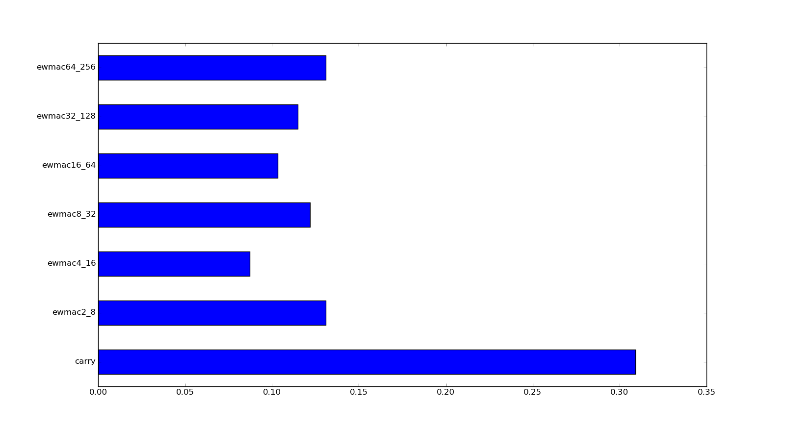
Let's first have a look at how each breakout rule looks across the whole portfolio of the six chapter 15 instruments. This charts use some code to disaggregate the performance of trading rules:
system.accounts.pandl_for_all_trading_rules_unweighted().to_frame()
There's a whole lot more of this kind of code, and if you're planning to use pysystemtrade it's probably worth reading this part of the manual (again).

Final thoughts
Ideally I'd now run the breakout rules together with the existing chapter 15 rules and see what the result is. However I already know from the correlation matrix and the account curves above that the answer is going to be a small improvement in performance from the ewmac+carry version, though probably not a significant one (I'm also in the middle of optimising pysystemtrade which runs far too slowly right now, to make such comparisons quicker).
Notice the difference in approach here. Traditionally a researcher would jump straight to the final backtest having come up with a rule to see if it works (and I confess, I've done that plenty of times in the past). They might then experiment to see which variation of breakout does the best. This is a shortcut on the road to over fitting.
Here I'm not even that interested in the final backtest. I know the rule behaves as I'd expect, and that's what's important. I'd be surprised if it didn't make money in the past; given it's designed to pick up on trends, and judging by it's correlation with ewmac does so very well. I have no idea whether there is a variation of breakout out of my set that is the best, or even if there is another combination of smooth and lookback that does even better.
Finally whether the rule will make money in the future is mostly down to whether markets trend or not.
Summary
I like the breakout rule, even if it turns out it was (sort of) invented by someone else. Diversifying by adding similar trading rules is never going to be the best way of diversifying your trading system. Doing something completely different like tactical short volatility, or adding instruments to your portfolio, are both better. The former does involve considerable work, and the latter involves some work and may also be problematic unless you have a 100 million dollar account.
But one of the advantages of being a fully automated trader is that adding variations is almost free; if you combine your portfolio in a linear way as I do it doesn't really affect your ability to interpret what the system is doing.
I'd rather have a large set of simple trading rules, even if they're all quite similar, than a smaller set of complex rules that has been potentially overfitted to death.


