Thursday 2 December 2021

My trading system

I realise that I've never actually sat down and described my fully automated futures trading system in all it's detail; despite having runit for around 7.5 years now. That isn't because I want to keep it a secret - far from it! I've blogged or written books about all the various components of the system. Since I've made a fair few changes to my  over the last year or so, it would seem to make sense to set down what the system looks like as of today.

You'll find reading this post much easier if you've already read my first book, "Systematic Trading". I'm expecting a christmas rush of book orders - I've bought all of my relatives copies, which I know they will be pleased to receive... for the 7th year in a row [Hope none of them are reading this, to avoid spoiling the 'surprise'!].


I'll be using snippets of code and configuration from my open source backtesting and trading engine, pysystemtrade. But you don't need to be a python or pystemtrade expert to follow along. Of course if you are, then you can find the full .yaml configuration of my system here. This code will run the system. Note that this won't work with the standard .csv supplied data files, since these don't include the 114 or so instruments in the config. But you can edit the instrument weights in the config to suit the markets you can actually trade.

In much of this post I'll also be linking to other blog posts I've written - no need to repeat myself ad infinitum.

I'll also be mentioning various data providers and brokers in this post. It's important to note that none of them are paying me to endorse them, and I have no connection with them apart from being a (reasonably) satisfied customer. In fact I'm paying them.... sadly.


Update: 5th January 2022, added many more instruments


Research summary

I basically had the same system from 2013 to the start of 2021, although in 2020 I did switch over the implementation to pysystemtrade from my legacy code (which wasn't open source.... because too ugly!). 

With my new dynamic system which I put into production about a month ago, which was a very significant change, I took the opportunity to look at all the research I'd done and see what was worth putting into the new system.

With that in mind I thought it might be fun to finish with a summary of the outcome of the various bits and bobs of research I've done in the last three years or so. 

Things I knew wouldn't work, but someone asked me to look at them:

Things I hoped would work, but didn't:

Things that worked, but I decided not to implement:

Things that worked and I did implement during 2021:

Having made these fairly serious changes to my system I don't plan on doing very much in the near future. I will however be looking at implementing some very different trading systems - watch this space.


Which markets should we sample / trade


I've already written about market selection at some length, here. But to summarise, here's the process I currently follow when adding new instruments:

  • Periodically survey the list of markets offered by my broker, interactivebrokers
  • Create a list of markets I want to add data for. Gradually work my way through them (as of writing this post, my wish list has 64 instruments in it!)
  • Regardless of whether I think I can actually trade them (see below), backfill their data using historic data from barchart.com
  • Add them to my system, where I will start sampling their prices
  • At this stage I won't be trading them until they're manually added to my system configuration

Because of the dynamic optimisation that my system uses, it's possible for me to calculate optimal positions for instruments that I can't / won't actually trade. And in any case, one might want to include such markets when backtesting - more data is always better! 

I do however ignore the following markets when backtesting:

  • Markets for which I have a duplicate (normally a different sized contract eg SP500 emini and micro; but could be a market traded in a different exchange) and where the duplicate is better. See this report.
  • A couple of other markets where my data is just a bit unreliable (I might delete these instruments at some point unless things improve)
  • The odd market which is so expensive I can't even just hold a constant position (i.e. the rolling costs alone are too much)

Then for trading purposes I ignore:

  • Markets for which there are legal restrictions on me trading (for me right now, US equity sector futures; but could be eg Bitcoin for UK traders who aren't considered MiFID professionals)
  • Markets which don't meet my requirements for costs and liqiuidity (again see here). This is why I sample markets for a while before trading them, to get an idea of their likely bid-ask spreads and hence trading costs
Again to reiterate, I can backtest these instruments and calculate optimal positions, I just won't actually take any positions.  Notice that I don't care here about contracts that are too big for me to trade; again my dynamic optimisation handles this. The size of contracts is only an issue 

There is some more pysystemtrade specific discussion of this here.

Note, if I wasn't using dynamic optimisation I'd use the methodology I discussed here to select a list of markets to trade, given my capital.


Which trading rules to use


I currently use the following trading rules:

Trend like:
  • Momentum - EWMAC (See my first or third book)
  • Breakout (blogpost)
  • Relative (cross sectional within asset class) momentum (blogpost)
  • Assettrend: asset class momentum (blogpost)
  • Normalised momentum (blogpost)
  • Acceleration 
Not trendy:
  • Slow mean reversion within an asset class 
  • Carry (See my first or third book)
  • Relative carry (blogpost)
  • Skewabs: Skew (blogpost)
  • Skew RV (blogpost)
  • Mean reversion in the wings

Some of these are not discussed in blogposts, but they will be in my forthcoming book (next year, hopefully - so that's Christmas 2022 sorted!).

All the code for these rules is here. Some of this duplicates example code elsewhere, but it's nicer to have it in one place.


Trading rule performance

Here are the crude Sharpe Ratios for each trading rule: 

breakout10      -1.19
breakout20 0.06
breakout40 0.57
breakout80 0.79
breakout160 0.79
breakout320 0.77
relmomentum10 -1.86
relmomentum20 -0.46
relmomentum40 0.01
relmomentum80 0.13
mrinasset160 -0.63
carry10 0.90
carry30 0.92
carry60 0.95
carry125 0.93
assettrend2 -0.94
assettrend4 -0.15
assettrend8 0.33
assettrend16 0.65
assettrend32 0.70
assettrend64 0.62
normmom2 -1.23
normmom4 -0.22
normmom8 0.41
normmom16 0.76
normmom32 0.82
normmom64 0.75
momentum4 -0.17
momentum8 0.46
momentum16 0.75
momentum32 0.78
momentum64 0.73
relcarry 0.37
skewabs365 0.52
skewabs180 0.42
skewrv365 0.22
skewrv180 0.33
accel16 -0.08
accel32 0.06
accel64 0.18
mrwrings4 -0.94

I say crude, because I've just taken the average performance weighting all instruments equally. In particular that means we might have a poor performance for a rule that trades quickly because I've used the performance from many expensive instruments which wouldn't actually have an allocation to that rule at all. I've highlighted these in italics. In bold are the rules that are genuine money losers:

  • mean reversion in the wings
  • mean reversion across assset classes

What these all have in common is they are non trendy, mean reverting, and hence highly diversifying rules. I haven't dropped them, because a proper handcrafting process would give them a positive weight: they are strongly negatively correlated to the trendy rules, and whilst their negative Sharpe Ratio tilts their allocation down a little, the uncertainty about backtested Sharpes means they are still justified a positive weighting.

Fun fact: If you could only trade one rule, I guess it would be carry. If you could trade two, well that would be carry and a slowish momentum


Vol attenuation

As discussed here for momentum like trading rules we see much worse performance when volatility rises. For these rules, I reduce the size of the forecast if volatility is higher than it's historic levels. The code that does that is here.


Forecast weights

I toyed with - and briefly implemented - the idea of fitting forecast weights in a rather complex way, but I've now reverted to the method I used to use: a very simple set of handcrafted weights (this is for live trading: when running proper backtests I still use an automated handcrafting method). The weights are as follows- working from the top down:

weights = dict(
trendy = 0.6,
other = 0.4)
# Level 2
weights = dict(
assettrend= 0.15,
relmomentum= 0.12,
breakout=    0.12,
momentum= 0.10,
normmom2= 0.11,
skew=        0.04,
carry= 0.18,
relcarry= 0.08,
mr= 0.04
accel= 0.06)
# Level 3
weights = dict(
assettrend2= 0.015,
assettrend4= 0.015,
assettrend16= 0.03,
assettrend32= 0.03,
assettrend64= 0.03,
assettrend8= 0.03,

relmomentum10= 0.02,
relmomentum20= 0.02,
relmomentum40= 0.04,
relmomentum80= 0.04,

breakout10= 0.01,
breakout20= 0.01,
breakout40= 0.02,
breakout80= 0.02,
breakout160= 0.03,
breakout320= 0.03,

momentum4= 0.005,
momentum8= 0.015,
momentum16= 0.02,
momentum32= 0.03,
momentum64= 0.03,

normmom2= 0.01,
normmom4= 0.01,
normmom8= 0.02,
normmom16= 0.02,
normmom32= 0.02,
normmom64= 0.03,

skewabs180= 0.01,
skewabs365= 0.01,
skewrv180= 0.01,
skewrv365= 0.01,

carry10= 0.04,
carry125= 0.05,
carry30= 0.04,
carry60= 0.05,

relcarry=         0.08,

mrinasset160= 0.02,
mrwrings4= 0.02,

accel16= 0.02,
accel32= 0.02,
accel64= 0.02
)

Next all I have to do is exclude any rules which a particular instrument can't trade because the costs exceed my 'speed limit' of 0.01 SR units. So here for example are the weights for an expensive instrument, Eurodollar with zeros removed:

EDOLLAR:
assettrend32: 0.048
assettrend64: 0.048
breakout160: 0.048
breakout320: 0.048
breakout80: 0.032
carry10: 0.063
carry125: 0.079
carry30: 0.063
carry60: 0.079
momentum32: 0.048
momentum64: 0.048
mrinasset160: 0.032
mrwrings4: 0.032
normmom32: 0.032
normmom64: 0.048
relcarry: 0.127
relmomentum80: 0.063
skewabs180: 0.016
skewabs365: 0.016
skewrv180: 0.016
skewrv365: 0.016

Forecast diversification multipliers will obviously be different for each instrument, and these are estimated using by standard method.


Position scaling: volatility calculation


As discussed here, I now estimate vol using a partially mean reverting method. The code for that is here. We use a combination of recent vol (70% weight) and vol averaged over the last 10 years (30% weight).


Instrument performance and characteristics

Of the 146 instruments in the dataset, 109 have positive Sharpe Ratios, with the median Sharpe Ratio coming in at 0.27.

The average correlation between subsystem returns is basically zero: 0.05. 


Instrument weights

Again, although in backtest I use an automated handcrafting, for live trading I prefer the weights I've built manually using just Excel. Not even Excel - just a pencil. Not even a pencil! A stick, and some mud! (that's enough, Ed). I won't paste in the weights here - lifes too short, but the weights by asset class are as follows:

{'Ags': 0.15, 
'Bond & STIR': 0.19, 
'Equity': 0.22, 
'FX': 0.13,
'Metals & Crypto': 0.13,
'OilGas': 0.13,
'Vol': 0.05}

The IDM is 2.5; somewhat below the estimated value (readers of Systematic Trading will know that I set a ceiling on this value of 2.5).


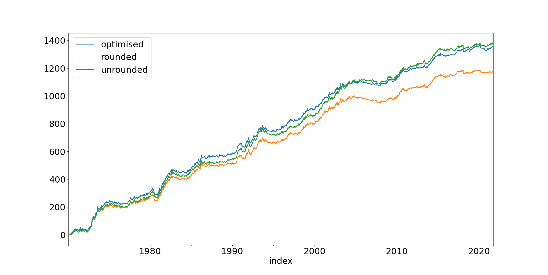
Dynamic optimisation


At this point I'll have a list of optimal positions in nearly 150 instruments. The vast majority of those will be less than one contract, because I don't have the tens of millions of dollars in my account that I'd need to actually consistently hold reasonable sized positions in all of those instruments.

As discussed here and here, the biggest change to my system this year has been the introduction of a dynamic optimisation system. This means I won't really have a position in 100+ instruments! I find the portfolio with the lowest tracking error to the optimal portfolio, accounting for the fact that we can only take integer contract positions. 

It's at this stage that I ignore instruments in the following categories when I do my optimisation:
  • Markets for which there are legal restrictions on me trading (for me right now, US equity sector futures; but could be eg Bitcoin for UK traders who aren't considered MiFID professionals)
  • Markets which don't meet my requirements for costs and liqiuidity (again see here)

As discussed in the blog post here, this is done using buffering to reduce trading costs.


Backtest properties

Let's finish with a look at the final backtest. Many words of warning here, since this backtest is stuffed full of in sample calibration and hence is likely to be massively better than you could realistically have expected. 


Looks nice, doesn't it? What about the daily returns?


So in case we were in any doubt 'black friday' (just on the end there) was indeed an exceptionally bad day. 

And drawdown:


Here are some stats. First daily returns:
('min', '-13.32'), ('max', '11.26'), ('median', '0.09578'), ('mean', '0.1177'), ('std', '1.44'), 
('ann_mean', '30.11'), ('ann_std', '23.04'), 
('sharpe', '1.307'), ('sortino', '1.814'), ('avg_drawdown', '-9.205'), 
('time_in_drawdown', '0.9126'), ('calmar', '0.7017'), ('avg_return_to_drawdown', '3.271'), 
('avg_loss', '-0.9803'), ('avg_gain', '1.06'), ('gaintolossratio', '1.081'), 
('profitfactor', '1.26'), ('hitrate', '0.5383'), 
('t_stat', '9.508'), ('p_value', '2.257e-21')

Now monthly:
[[('min', '-21.84'), ('max', '45.79'), ('median', '2.175'), ('mean', '2.55'), 
('std', '7.768'), ('skew', '0.9368'), ('ann_mean', '30.55'), ('ann_std', '26.91'), 
('sharpe', '1.135'), ('sortino', '2.177'), ('avg_drawdown', '-5.831'), 
('time_in_drawdown', '0.6485'), ('calmar', '0.8371'), 
('avg_return_to_drawdown', '5.239'), ('avg_loss', '-4.465'), ('avg_gain', '6.741'), 
('gaintolossratio', '1.51'), ('profitfactor', '2.527'), 
('hitrate', '0.626'), ('t_stat', '8.193'), ('p_value', '1.457e-15')]

Oh, and costs come in at a very reasonable 1.06% a year: well below my speed limit (1.06 / 25 = 0.042 SR units)


So....

Any questions are welcome as usual. If you want to get into an extended discussion, it's probably best to do so here.

Otherwise it's just for me to wish you all (as this is my last blog post of the year) a merry christmas, a happy new year, and let's all hope that 2022 is an improvement on the previous couple of years.


Postscript (6th December 2021)


I thought it might be interesting to compare my backtested results with live trading. Of course, these are very different systems - until the last couple of weeks or so - but it's still interesting.


Friday 19 November 2021

Mr Greedy and the Tale of the Minimum Tracking Error Variance - Part two

My last blog post was about a new method for a daily dynamic optimisation of portfolios with limited capital, to allow them to trade large numbers of instruments. 

(Although I normally write my blog posts to be self contained, you'll definitely have to read the previous one for this to make any sense!)

Subsequent to writing that post I implemented the method, and quickly ran into some problems. Basically the dammn thing was trading too much. Fortunately there is a single parameter which controls trading speed in the model - the shadow cost. I turned up the shadow cost to a very high value and spent a few days investigating what had went wrong.

Broadly speaking, I found that:

  • My measure of turnover wasn't suitable for 'sparse' portfolios, i.e. portfolios where most instruments have a zero position at any given time
  • My measure of risk adjusted costs also wasn't suitable
  • The true turnover of the dynamic optimised portfolio was much higher than I'd realised
  • The true trading costs were thus also much higher
  • Thus the results in my previous post were misleading and wrong

After discussing with Doug (the original source of this idea) I realised I'd been missing a step: postion buffering. This is something I did in my original static system to slow down my trading behaviour, but which was missing here. 

In this post I explain:

  • Some other bad things I did
  • Why my approximations for trading costs and turnover were wrong, and how I fixed them
  • Why increasing the shadow cost doesn't help
  • Why position buffering is a good thing and how it works in the old 'static' system
  • How to create a position buffering method for dynamic optimisation
  • How I calibrated the position buffering and shadow cost for the dynamic model
  • How I used shrinkage to make the results more stable
  • A more appropriate benchmark
  • Some revised results using the new method, and more accurate statistics

So there's a lot there, but this has been quite an extensive (and at times painful!) piece of research.


Some other bad things I did


As well as the stuff I've already mentioned I did some bad things when implementing the model to production. I was so excited about the concept, basically I rushed it. Here's a list of things I did:

  • Not thinking more carefully about the interpretation of the shadow cost
  • Not using common code between sim and production (this didn't serious cause problems, but did make it harder to work out what was going ong)
  • Not paper trading for long enough
I ought to know better, so this just goes to show that even supposedly experienced and smart people make mistakes...


My (bad) approximations for trading costs and turnover


I'm a big fan of using risk adjusted measures for trading costs and other things. Here's how I used to work out trading costs:

  • Work out the current cost of trading
  • Divide that by current vol to calculate the cost in SR units
  • Calculate the turnover in contracts
  • Calculate the normalised turnover; dividing the historic turnover in contracts by the current average position, and the taking an average
  • The average position assumes we have a constant forecast of +10
  • Multiply the normalised turnover
  • I do a similar calculation for rolling costs, assuming I roll an average position worth of contracts N times a year (where N is the number of rolls each year)
The big flaw in this, with respect to sparse positions, is the average position. Clearly our average position is going to be much smaller than we think, which means our turnover will look unnaturally low, and our costs unrealistically low.

  • Work out the current cost of trading in actual $$$ terms
  • For each historic trade, multiply that by the number of contracts traded
  • For rolling costs, assume we roll a number of contracts equal to the number of contracts we held in the period before the roll (gives a more reliable figure)
  • Deflate these figures according to the difference in price volatility between then and now
  • So for example, if the vol of S&P 500 is 20% with a price of 5000, that's a price vol of 1000
  • If that figure was 200 at some point in the past, then we'd divide the historic cost by 5
This still risk adjusts costs, but in such a way that it will reflect sparse positions.

(Incidentally, I still use the old SR based method to calculate the cost of a trading rule, for which we don't really know the exact number of contracts)

We don't use turnover anymore, but it would still be nice to know what it is. It's hard to calculate a turnover per instrument with sparse positions, but we can meaningfully calculate the turnover for an entire system. We do this by calculating the turnover in contracts at the portfolio level (after dynamic optimisation, or after buffering for the static system), divide each of these by the expected average position (assuming a forecast of +10, and accounting for instrument weights and IDM), and then add these up. 


Why shadow cost doesn't help - much


So when I first calculated this new measure of average turnover for the dynamic system, it was quite a bit higher than I expected.

"No problem" I thought "I'll increase the shadow cost".

Remember the shadow cost is a multiplier on the cost penalty applied to the dynamic optimisation. Increasing it ought to slow the system down.

And it does... but not by as much as I'd hoped, and with a decreasing effect for higher shadow costs. Digging under the hood of the greedy algo, the reason for this is that the algo always starts at zero (in the absence of corner case constraints) and then starts changing position with the sign of the optimal unrounded position

So it will always end up with the same sign of position as the underlying optimal position. To put it another way, every time the underlying forecast changes sign, we'll definitely trade regardless of the size of the shadow cost. All the shadow cost will do is reduce trading in instruments where we haven't seen a sign change.

No biggie, except for the uber-portfolio I was running in production with over 110 instruments. Let's say their average holding period is a conservative two months; so they change sign roughly every 42 business days. That means on any given day we'd see around three instruments changing sign, and trading. This imposes a lower limit on turnover, no matter how much you crank up the shadow cost. 

There isn't a lot you can do about this, except perhaps switch to a different optimisation method. I did look at this, but I really like the intuitive behaviour of the greedy algo.

Another - smaller - effect is that the more instruments you have, the higher your IDM, the higher your turnover will be (as a rule of thumb, if you double your leverage on an individual instrument, you'll also double your turnover).

So it's important to do any testing with a sufficiently large portfolio of instruments relative to capital.


Position buffering in a static system


Anyway the solution, after discussion with Doug, revolves around something in my old 'static' system that's missing from the new dynamic system: position buffering. 

Doug isn't doing exactly what I've decided to do, but the principal of applying a buffer was his idea so is due credit

Position buffering works something like this; suppose we calculate an optimal (unrounded) position of long +2.3 contracts (2 contracts rounded). We then measure a buffer around this; which for the sake of argument we'll say is 2 contracts wide. So the position plus buffer will be (lower level) 1.3 contracts to (upper level) 3.3 contracts. Rounded that's +1 to +3 contracts. 

We then compare this to our current position. If that's between 1 and 3, we're good. We do nothing. However let's suppose our current position is +4 contracts. Then we'd sell... not 2 contracts bringing us back to the (rounded) optimal of +2, but instead a single contract to bring us to +3... the edge of the buffer.

Buffering reduces our turnover without affecting our performance, as long as the buffer isn't too wide. Calibrating the exact width of the buffer is quite involved (it's related to the interplay of forecast speed and costs for a given instrument), so I've always used a simple 10% of average position (the position I'd get with an average forecast of +10).


Position buffering in a dynamic system


How do we impose a buffer on the dynamic system? We could try and set up the optimisation so it treats all positions within the buffer for each instrument as having the same utility... but that would be darned messy. And as we're not doing a grid search which tests every possible integer contract holding we wouldn't neccesarily use the buffer in a sensible way.

Instead we need to do the buffering at a portfolio level. And we'll do the buffering on our utility function: the tracking error.

So the basic idea is this: if the tracking error of the current portfolio is less than some buffer level, we'll stick with the current portfolio (='inside the buffer'). If it isn't, we'll trade in such a way to bring our tracking error down to the buffered level (='trading to the edge of the buffer').

We actually do this as a three step process. In step one we calculate the tracking error of the current portfolio, versus the portfolio with unrounded optimal positions (let's call this tracking error /unrounded). If this is less than the buffer, we stick with the current positions. No optimisation is needed. This step doesn't affect what happens next, except to speed things up by reducing the number of times we need to do a full blown optimisation.

Step two: we do the optimisation, which gives a portfolio consisting of integer positions. Step three: we now calculate a second tracking error: the tracking error of the currently held portfolio versus the integer positions (tracking error/rounded). By construction, this tracking error will be lower than tracking error/unrounded. 

We now calculate an adjustment factor, which is a function of tracking error/rounded (which I'm now going to rename x) and the buffer (b):

Adjustment factor = max((x - b)/x, 0)

We then multiply all our required trades (from current to integer optimised) by the adjustment factor. And then round them, obviously.

So if the tracking error is less than the buffer, we don't trade. Otherwise we do a proportion of the required trade. The further away we are from the buffer, the more of the trade we'll do. For a very large x, we'd do almost all of our trade.

Note that (ignoring the fact we need to round trades) doing this will bring our tracking error back to the edge of the buffer.


Calibrating buffer size and shadow cost


Note the buffer doesn't replace the shadow cost; it's in addition to it. The shadow cost is handy since it penalises the costs of trading according to the different costs of each instrument. Nevertheless, both methods will slow down our trading so we have to consider their joint effect.

We could do this with an old school, in sample, grid search of parameters. Instead let's use some common sense.

Firstly, with an average target risk of 25%, a 10% buffer around that means our dynamic buffer size should be around 1.25% (not 2.5% as you might expect as this buffer is expressed differently).

Now consider the shadow cost. In my prior post I said that a shadow cost of 10 'looked about right', but a few moments thought reveals it is not. Remember the utility function is tracking error - costs. Tracking error is measured in units of annualised standard deviation. How much does a tracking error of 1% lose use in terms of expected return? Difficult to say, but let's make some assumptions:

  • Sharpe Ratio 1.0
  • Target annual standard deviation 25%
  • Target annual return = 1.0 * 25% = 25%
  • Suppose we're running at half the risk we want, so our tracking error will be 12.5%
  • In this case we'll also be missing out on ~12.5% of annual return
  • If SR = 1, then tracking error is effectively in annualised return units
Now bear in mind the utility function subtracts the cost from a given optimisation; which is probably a daily cost, we need to annualise this. So a shadow cost of 250 would annualise costs and put them in the same units as the tracking error.

To recap then:

- Shadow cost 250
- Buffer size 0.0125


Shrinkage and the mystery of the non semi-definite matrix


In the discussion 'below the line' of the previous post it was suggested that the turnover in the correlation matrix might be responsible for the additional costs. Basically, if the correlation estimate was to change enough it would cause the optimal portfolio to change a lot as well.

It was suggested to try shrinking the correlation matrix, which would result in fewer correlation changes. But the correlation estimate is also quite slow so I didn't shrinkage would be worthwhile. However I then discovered another problem, which led me down quite the rabbit hole. 

Essentially, once I started examining the results of my optimisation more carefully, I realised that for large (100+ instrument) portfolios there were instances when my optimisation just broke as it couldn't evaluate the utility function. One cause was inputting costs of nan, and was easily fixed by making my cost deflation function more accurate. But I also got errors trying to find the standard deviation of the tracking error portfolio. 

So it turns out that pandas doesn't actually guarantee to produce positive semi-definite correlation matrices, which means that sometimes the tracking error of the portfolio can have a negative variance. I experimented with trying to find the nearest PSD matrix - it's very slow, too slow for backtesting though possibly worth a last line of defence. I tried tweaking the parameters of the exponential correlation; even tried going back to vanilla non exponential correlation estimates but still ended up with non PSD matrices. 

What eventually came to the rescue, just as I was about to give up, was shrinking the correlation matrix. For reasons that are too boring to go into here (but try here), shrinkage is a good way of fixing PSD issues. And shrinking the correlation matrix in this particular application isn't really a bad thing. It makes it less likely we'll put on weird positions, just because correlations are especially high or low.

(If anyone has come across this problem with pandas, and has a solution, I'd like to hear it...)


How should we assess this change?


Yet another flaw in the previous post was an excessive reliance on looking at Sharpe Ratios to see if performance improved, comparing a plain 'rounded' with an optimised portfolio. 

However, there is an element of luck involved here. For example, if there was an instrument with a low contract size which still had positions even for a small unoptimised portfolio, and which had a higher SR than anything else, then the simple rounded portfolio would outperform the optimised portfolio. 

A better set of metrics would be:
  • The correlation in returns between an unrounded and the rounded optimised portfolio
  • The level of costs paid in SR units
  • The total portfolio level turnover (see notes above)
We'd want to check the SR wasn't completely massacred by the dynamic optimisation, but a slight fall in SR isn't a go/no go decision.


The static benchmark

It could be argued that a better benchmark would not be the simple rounded static portfolio with say 100 instruments; but instead the 30 or so instrument static portfolio you'd actually be able to trade with say $500K in your account. Again, there is an element of luck here, depending on which set of 30 or so instruments you choose. But it would give a good indication of what sort of turnover we are aiming for, and whether we had the costs about right.

So I reran the process described here, and came up with the following list of static instruments for a $500K portfolio:

instrument_list = ['DOW', 'MUMMY','FTSECHINAA', 'OAT',  'NIFTY', 'KOSDAQ','SP500_micro', 'NIKKEI',
'BOBL', 'KR10','KR3','EDOLLAR', 'US10U','US3',
'SOYOIL',
'WHEAT', 'LIVECOW', 'LEANHOG',
'CNH', 'YENEUR','RUR','BRE', 'JPY', 'MXP', 'NZD','CHF',
'BITCOIN', 'IRON','SILVER', 'GOLD_micro' ,
'CRUDE_W_mini', 'GASOILINE','GAS_US_mini',
'VIX'
]
Notice I've grouped these by asset class:
  • Equities
  • Bonds/STIR
  • Ags
  • Currencies
  • Metals
  • Energies
  • Vol
The results are different from last time, as I've added more instruments to my data set, and also excluded some instruments which are too expensive / illiquid; having spent some time recently on putting together a systematic process for identifying those.

For benchmarking purposes I allowed the instrument weights to be fitted in both dynamic and static cases, however both sets of portfolios have forecast weights that are fitted in sample for speed.


Results versus benchmark


First let's get a feel for the set of instruments we are playing with. We have 114 instruments in total, reflecting my constantly expanding universe, with data history that looks like this:

For the 34 instruments in the benchmark portfolio, it's worth bearing in mind that prior to 2000 we have less than 15 instruments, and so the early part of the backtest might be worth a pinch or two of salt:


Now in reality we can't hold 114 instruments at once, so in the dynamic optimised portfolio we end up holding around a quarter to a third of what's available on any given day:


Whilst in the benchmark portfolio we mostly hold positions in around 90-100% of what we can trade:

Let's dig into the optimiser some more and make sure it's doing it's job. Here is the position series for the S&P 500 micro. The blue line shows the position we'd have on without rounding. Naturally the green buffered position follows this quite closely. We actually end up with the orange line after optimisation; it follows along but at times clearly prefers to get it's risk from elsewhere. This is a cheap future so the turnover is relatively high:

Another plot I used in the previous post was to see how closely the expected risk tracked between the unrouded and optimised portfolio. It's still a very close match:
Remember one of our key metrics was the return correlation between the unrounded and optimised portfolios. This comes in at a very unshabby 0.986.

Let's look at some summary statistics. The Sharpe Ratio of the optimised portfolio is 1.336 gross, 1.287 net. So that's a SR cost loss of ~5bp a year. In other words, we'd expect to lose 1/20 of our vol target (1/20 of 25% = 1.25%) in costs annually; the actual average cost is 1.7% a year. The portfolio level turnover is 51.1 times a year. 

In comparison the benchmark portfolio hits a Sharpe Ratio of gross 1.322, net 1.275, SR in costs again ~5bp. Actual average cost is slightly lower at 1.45% a year. Turnover is 37.5. I'll discuss those figures in more detail later.

Incidentally, the (unachievable!) Sharpe Ratio of the unrounded portfolio with 114 instruments is 1.359. So we're only losing a few bp in SR when holding about a quarter to a third of the available instruments. You can see how close the account curves are here:
Orange: Unrounded, Blue: Optimised

Another way of visualising the costs: If I plot the costs with the sign flipped, and multiplied by 10, and then add on the net account curve; you can see how we are losing less than half  (so less than 5%) of our gross performance. Also the compounded costs are steady and linear, indicating a nice consistency over time.

Let's compare that to the benchmark:


Although the proportion of costs is slightly lower, you can see here that costs have increased over time. And in fact the annual costs over the last 15 years have been around 2%: higher than the 1.7% achieved by the dynamic system. 

So if we're comparing dynamic with static benchmark:

  • In recent years it has lower costs
  • But probably higher turnover
  • The historic net Sharpe Ratio is effectively identical

The turnover isn't a massive deal, as long as we have accurately estimated our trading costs: we'll do a few more trades, but on average they will be in cheaper markets.

However, to reiterate, the results of the static system are very much more a matter of luck in market selection particularly for the early backtest when it only has a few markets. Overall I'd still rather have the dynamic system - with the opportunity to catch market movements in over 100 markets and counting - than the static system where if I am missing a market that happens to move I will kick myself.


Summary

"I've prodded and poked this methodology in backtesting, and I'm fairly confident it's working well and does what I expect it to." ....

.... is something I wrote in my last post. And I was wrong! However, after a lot more prodding and poking, which has had the side effect of tightening up a lot of my backtesting framework and making me think a lot, I'm now much more confident. And indeed this system is now trading 'live'.

That was the seventh post on the best way to trade futures with a small account size, and - barring another unexpected problem - that's all folks!


Friday 1 October 2021

Mr Greedy and the Tale of the Minimum Tracking Error Variance [optimising portfolios for small accounts dynamic optimisation testing / yet another method!]

 This is the sixth (!) post in a (loosely defined) series about finding the best way to trade futures with a relatively small account size.

  • This first (old) post, which wasn't conciously part of a series, uses an 'ugly hack': a non linear rescaling of forecasts such that we only take positions for relatively large forecast size. This is the method I was using for many years.
  • These two posts (first and second) discuss an idea for dynamic optmisation of positions. Which doesn't work.
  • This post discusses a static optimisation method for selecting the best set of instruments to include in a system given limited capital. This works! This is the method I've been using more recently.
  • Finally, in the last post I go back to dynamic optimisation, but this time using a simpler heuristic method. Again, this didn't work very well.
(Incidentally, if you're new to this problem, it's probably worth reading the first post on dynamic optimisation post in my series

That would be the end of the story, apart from the fact that I got a mysterious twitter reply:


After some back and forth I finally got round to chatting to Doug in mid September. Afterwards, Doug sent me over some code, which was in R, a language I haven't used for 14 years but I did manage to translate it into Python and then integrate it into https://github.com/robcarver17/pysystemtrade, and added in some variations of my own (more realistic costs, and some constraints for use in live trading). Then I tested it. And blimey, it actually bloody worked.


UPDATE (22nd October 2021) 

It didn't work, at least not as well as I'd hoped.

After writing this post and implementing the idea in production I found some issues in my backtesting results were producing misleading results (in short my cost calculations were not appropriate for a system with 'sparse' positions - there is more detail here). 

I could rewrite this post, but I think it's better to leave it as a monument to my inadequacy. I'm working on an alternative version of this method that I hope will work better.


UPDATE (November 2021) 
The alternative version is here. This is now what I use in production.


What was Doug's brilliant idea


Doug's idea had two main insights:
  • It's far more stable to minimise the variance of the tracking error portfolio, rather than using my original idea (maximising the utility of the target portfolio, having extracted the expected return from the optimal portfolio). And indeed this is a well known technique in quant finance (people who run index funds are forever minimising tracking error variance).
  • A grid search is unneccessary given that in portfolio optimisation we usually have a lot of very similar portfolios, all of which are equally as good, and finding the global optimum doesn't usually give us much value. So using a greedy algorithm is a sufficiently good search method, and also a lot faster as it doesn't require exponentially more time as we add assets.

Mr Greedy
https://mrmen.fandom.com/wiki/Mr._Greedy?file=Mr_greedy_1A.png


Here's the core code (well my version of Doug's R code to be precise):

def greedy_algo_across_integer_values(
obj_instance: objectiveFunctionForGreedy
) -> np.array:

## Starting weights
## These will eithier be all zero, or in the presence of constraints will include the minima
weight_start = obj_instance.starting_weights_as_np()

## Evaluate the starting weights. We're minimising here
best_value = obj_instance.evaluate(weight_start)
best_solution = weight_start

done = False

while not done:
new_best_value, new_solution = _find_possible_new_best(best_solution = best_solution,
best_value=best_value,
obj_instance=obj_instance)

if new_best_value<best_value:
# reached a new optimium (we're minimising remember)
best_value = new_best_value
best_solution = new_solution
else:
# we can't do any better (or we're in a local minima, but such is greedy algorithim life)
break

return best_solution


def _find_possible_new_best(best_solution: np.array,
best_value: float,
obj_instance: objectiveFunctionForGreedy) -> tuple:

new_best_value = best_value
new_solution = best_solution

per_contract_value = obj_instance.per_contract_value_as_np
direction = obj_instance.direction_as_np

count_assets = len(best_solution)
for i in range(count_assets):
temp_step = copy(best_solution)
temp_step[i] = temp_step[i] + per_contract_value[i] * direction[i]

temp_objective_value = obj_instance.evaluate(temp_step)
if temp_objective_value < new_best_value:
new_best_value = temp_objective_value
new_solution = temp_step

return new_best_value, new_solution

Hopefully that's pretty clear and obvious. A couple of important notes:

  • The direction will always be the sign of the optimal position. So we'd normally start at zero (start_weights), and then get gradually longer (if the optimal is positive), or start at zero and get gradually shorter (if the optimal position is a negative short). This means we're only ever moving in one direction which makes the greedy algorithim work. Note: This is different with certain corner cases in the presence of constraints. See the end of the post.
  • We move in steps of per_contract_value. Since everything is being done in portfolio weights space (eg 150% means the notional value of our position is equal to 1.5 times our capital: see the first post for more detail), not contract space, these won't be integers; and the per_contract_value will be different for each instrument we're trading.

Let's have a little look at the objective function (the interesting bit, not the boilerplate). Here 'weights_optimal_as_np' are the fractional weights we'd want to take if we could trade fractional contracts:


class objectiveFunctionForGreedy:
    ....
def evaluate(self, weights: np.array) -> float:
solution_gap = weights - self.weights_optimal_as_np
track_error = \
(solution_gap.dot(self.covariance_matrix_as_np).dot(solution_gap))**.5

trade_costs = self.calculate_costs(weights)

return track_error + trade_costs

def calculate_costs(self, weights: np.array) -> float:
if self.no_prior_weights_provided:
return 0.0
trade_gap = weights - self.weights_prior_as_np
costs_per_trade = self.costs_as_np
trade_costs = sum(abs(costs_per_trade * trade_gap * self.trade_shadow_cost))

return trade_costs

The tracking error portfolio is just the portfolio whose weights are the gap between our current weights and the optimal unrounded weights, and what we are trying to minimise is the standard deviation of that portfolio.

The covariance matrix used to calculate the standard deviation is the one for instrument returns (not trading subsystem returns); if you've followed the story you will recall that I spent some time grappling with this decision before and I see no reason to change my mind.  For this particular methodology the use of instrument returns is a complete no-brainer.

The shadow cost is required because portfolio standard deviation and trading costs are in completely different units, so we can't just add them together. It defaults to 10 in my code (some experimentation reveals roughly this value gives the same turnover as the original system before the optimisation occurs. As you'll see later I haven't optimised this for performance).


Performance


And let's have a look at some results (45 instruments, $100K in capital). All systems are using the same basic 3 momentum crossover+carry rules I introduce in chapter 15 of my first book.


So if we were able to take fractional positions (which we're not!) we could make the green line (which has a Sharpe Ratio of 1.17). But we can't take fractional positions! (sad face and a Sharpe Ratio of just 1.06). But if we run the optimiser, we can achieve the blue line, even without requiring fractional positions. Which has a Sharpe Ratio of .... drumroll... 1.19. 

Costs? About 0.13 SR units for all three versions.

Tiny differences in Sharpe Ratio aside, the optimisation process does a great job in getting pretty close to the raw unrounded portfolio (correlation of returns 0.94). OK the rounded portfolio is even more correlated (0.97) , but I think that's a price worth paying.

That's a little higher than what you will have seen in previous backtests. The reason is I'm now including holding costs in my calculations. I plan to exclude some instruments from trading whose holding costs are a little high, which will bring these figures down, but for now I've left them in.

If I do a t-test comparing the returns of the three account curves I find that the optimised version is indistinguishable from the unrounded fractional position version. And I also find that the optimised version is significantly better than the rounded positions: a T-statistic of 3.7 with a tiny p-value. Since these are the versions we can actually run in practice, that is a stonking win for the optimisation.


Risk


The interesting thing about the greedy algorithm is that it gradually adds risk until it finds the optimal position, whilst trying to reduce the variance of the delta portfolio, so it should hopefully target similar risk. Here is the expected (ex-ante) risk for all three systems:

Red line: original system with rounded positions, Green line: original system with unrounded positions, Blue line: optimised system with unrounded positions


It's quite hard to see what's going on there, so let's zoom into more recent data:


You can see that the optimiser does a superb job of targeting the required risk, compared to the systematically under-risked (in this period - sometimes it will be over-risked) and lumpy risk presented by the rounded positions. The ex-post risk over the entire dataset comes in at 22.4% (unrounded), 20.9% (rounded) and 21.6% (optimised); versus a target of 20%. 


How many positions do we typically take?


An interesting question that Doug asked me is how many positions the optimiser typically takes.

"Curious how many positions it uses of the 45??

I guess I don’t know how much capital you are running, but given there are really only maybe 10 independent bets there (or not many more) does it find a parsimonious answer that you might use even if you had a giant portfolio to run?"

Remember we have 45 markets we could choose from in this setup, how many do we actually use?

Blue line: Total number of instruments with data. Orange line: Instruments with positions from optimiser


The answer is, not many! The average is 6, and the maximum is 18; mostly it's less than 12. And (apart from at the very beginning) the number of instruments chosen hasn't increased as we add more possible instruments to our portfolio. Of course we couldn't really run our system with just 12 instruments, since the 12 instruments we're using varies from period to period. But as Doug notes (in an email):

"Pretty cool. The dimension of the returns just isn’t all that high even though there are so many things moving around." 

Interestingly, here are some statistics showing the % of time any given instrument has a position on. I've done this over the last 7 years, as otherwise it would be biased towards instruments for which we have far more data:

PALLAD          0.00
COPPER          0.00
GASOILINE       0.00
FEEDCOW         0.00
PLAT            0.00
HEATOIL         0.00
GBP             0.01
REDWHEAT        0.02
WHEAT           0.02
EUR             0.02
NZD             0.03
CRUDE_W_mini    0.03
US20            0.03
US10            0.03
SOYOIL          0.04
LEANHOG         0.04
AUD             0.04
LIVECOW         0.05
JPY             0.05
SOYMEAL         0.06
CAC             0.07
SOYBEAN         0.08
OATIES          0.08
OAT             0.09
RICE            0.10
US5             0.11
MXP             0.12
CORN            0.13
BTP             0.14
SMI             0.14
AEX             0.14
GOLD_micro      0.19
EUROSTX         0.23
KR10            0.24
BITCOIN         0.26
EU-DIV30        0.33
BUND            0.39
EDOLLAR         0.39
BOBL            0.43
NASDAQ_micro    0.47
VIX             0.55
SP500_micro     0.60
KR3             0.66
US2             0.73
SHATZ           0.74


Notice we end up taking positions in all but six instruments. And even if we never take a position in those instruments, their signals are still contributing to the information we have about other markets. Remember from the previous posts, I may want to include instruments in the optimisation that are too illiquid or expensive to trade, and then subsequently not take positions in them.

I've highlighted in bold the 16 instruments we trade the most. You might want to take the approach of only trading these instruments: effectively ignoring the dynamic nature of the optimisation and saying 'This is a portfolio that mostly reproduces the exposure I want'. 

However notice that they're all financial instruments (Gold and Bitcoin, quasi financial), reflecting that the big trends of the last 7 years have all been financial. So we'd probably want to go further back. Here are the instruments with the most positions over all the data:

PLAT            0.24
RICE            0.25
CRUDE_W_mini    0.26
NASDAQ_micro    0.27
SOYMEAL         0.33
US2             0.35
US5             0.38
WHEAT           0.39
LIVECOW         0.40
LEANHOG         0.41
CORN            0.43
SOYOIL          0.44
EDOLLAR         0.46
SP500_micro     0.56
GOLD_micro      0.56
OATIES          0.61

That's a much more diversified set of instruments. But I still don't think this is the way forward.


Tracking error


Tracking error: I like to think of as quantified regret. Regret that you're missing out on trends in markets you don't have a full size position in...

What does the tracking error look like? Here are the differences in daily returns between the unrounded and optimised portfolio:

The standard deviation is 0.486%. It also looks like the tracking error has grown a little over time, but 2020 aside it has been fairly steady for a number of years. My hunch is that as we get more markets in the dataset it becomes more likely that we'll have fractional positions in a lot of markets that the optimiser can't match very well. And indeed, if I plot the tracking error of rounded versus unrounded portfolios, it shows a similar pattern. The standard deviation for that tracking error is also virtually identical: 0.494%. 


Checking the cost effects


It's worth checking to see what effect the cost penalty is having. I had a quick look at Eurodollar, since we know from the above analysis that it's a market we normally have a position on. Zooming in to recent history to make things clearer:


The green line is the unrounded position we'd ideally want to have on, wheras the red line shows our simple rounded (and buffered) position. The blue line shows what the optimiser would do without a cost penalty. It trades - a lot! And the orange line shows our optimised position. It's trading a bit more than the red line, and interestingly often has a larger position on (where it's probably taking on more of the load of being long fixed income from other instruments), but it's definitely trading a lot less than the blue line.

Interestingly the addition of the cost penalty doesn't reduce backtested costs much, and reduces net performance a little: about 1 SR point, but I'd still rather have the penalty thanks very much. 


Much lower capital

To ssee how robust this approach is, let's repeat some of the analysis above with just 50K in capital. 


So the optimised version is still better than the rounded (SR improvement around 0.1), but nowhere near as good as the unrounded (SR penalty around 0.2). We can't work miracles! With 50K we just don't have enough capital to accurately reflect the exposures we'd like to take in 45 markets. The tracking error vs the unrounded portfolio is 0.72% for the optimiser (versus 0.49% earlier with 100K), but is even higher for the rounded portfolio (0.76%). The correlation between the optimiser and ideal unrounded optimal returns has dropped to 0.86 (0.94 with 100K); but for rounded positions is even lower: 0.84 (0.97 with 100K).

Less capital makes it harder to match the unrounded position of a large portfolio of instruments, but relatively speaking the dynamic optimisation is still the superior method.

Important note: With 


What does this mean?

Let's just review what our options are if we have limited capital, of say $100K:
  • We could win the lottery and trade the unrounded positions.
  • We could try and trade a lot of instruments - say 45 - and just let our positions be rounded. This gives us a SR penalty of around 0.1 SR versus what we could do with unrounded positions. The penalty would be larger (in expectation) with less capital and / or more instruments (eg it's 0.3SR with 50k). The tracking error would also get larger for smaller capital, relative to the number of instruments.
  • We could try and choose a set of static instruments and just trade those. In this post I showed that we could probably choose 16 instruments using a systematic approach. This would also give us a SR penalty of around 0.1 SR in expectation, but the tracking error would be larger than for rounded positions. Again with less capital / more instruments both penalties and tracking error would be larger.
  • We could use the 'principal components' approach, to choose a static list of the 16 instruments that are normally selected by the optimiser. I've highlighted these in the list of instruments above. Our tracking error would be a little smaller (in expectation) than for rounded positions, but we'd still have a SR penalty of around 0.1 SR.
  • We could have as many instruments as we liked in our portfolio and use the dynamic optimisation approach to decide which of those to hold positions for today. Normally this means we'll only have positions in around 10 instruments or so, but the 10 involved will change from day to day. Our tracking error would be similar as for rounded positions, but we'd not be giving up much in terms of SR (if anything). With smaller capital or more instruments we'd get some SR penalty (but less than the alternatives), and higher tracking error (but again better than the alternatives). 
Ignoring the first option, it strikes me that dynamic optimisation brings significant benefits, which for me overcome the additional complexity it introduces into our trading.


Live trading


If you're clever, you will have noticed that the algo code above doesn't include any provision for some of the features I specified in my initital post on this subject:

  • A 'reduce only' constraint, so I can gradually remove instruments which no longer meet liquidity and cost requirements
  • A 'do not trade' constraint, if for some reason 
  • Maximum position constraints (which could be for any reason really) 
The psystemtrade version of the code here covers these possibilities. It adjusts the starting weights and direction depending on the constraints above, and also introduces minima and maxima into the optimisation (and prevents the greedy algorithim from adjusting weights any further once they've hit those). It's a bit complicated because there are quite a few corner cases to deal with, but hopefully it makes sense.

Note: I could use a more exhaustive grid search for live trading, which only optimises once a day, but I wouldn't be able to backtest it with 100+ instruments so I'll stick with the greedy algorithim, which also has the virtue of being a very robust and stable process and avoids duplicating code.

Let's have a play with this code and see how well it works. Here's what the optimised positions are for a particular day in the data. In the first column is the portfolio weight per contract. The previous days portfolio weights are shown in the next column. The third column shows the optimal portfolio weights we'd have in the absence of rounding. The optimised positions are in the final column. I've sorted by optimal position, and removed some very small weights for clarity:

              per contract  previous  optimal  optimised
SHATZ 1.32 -10.56 -3.08 -5.27
BOBL 1.59 -1.59 -1.09 0.00
OAT 1.97 0.00 -0.31 0.00
VIX 0.24 0.00 -0.14 -0.24
EUR 1.47 0.00 -0.13 0.00
... snip...

GOLD_micro 0.18 0.00 -0.01 -0.18
... snip...

AEX 1.84 1.86 0.12 0.00
EUROSTX 0.48 0.00 0.13 0.48
EU-DIV30 0.22 0.22 0.14 0.00
MXP 0.25 0.00 0.16 0.00
US10 1.33 1.33 0.17 1.33
SMI 1.27 0.00 0.19 0.00
SP500_micro 0.22 0.00 0.21 0.00
US20 1.64 0.00 0.23 0.00
NASDAQ_micro 0.30 0.31 0.26 0.30
US5 1.23 2.47 0.33 2.47
KR10 1.07 0.00 0.41 0.00
BUND 2.01 0.00 0.91 0.00
EDOLLAR 2.47 0.00 1.44 0.00
KR3 0.94 3.77 2.96 3.77
US2 2.20 8.81 17.44 8.81

Now let's suppose we could only take a single contract position in US 5 year bonds, which is a maximum portfolio weight of 1.23:

              weight per contract  previous  optimal  optimised  with no trade
SHATZ 1.32 -10.56 -3.08 -5.27 -2.63
BOBL 1.59 -1.59 -1.09 0.00 0.00
OAT 1.97 0.00 -0.31 0.00 0.00
VIX 0.24 0.00 -0.14 -0.24 -0.24
... snip...
GOLD_micro                   0.18      0.00    -0.01      -0.18           0.00
... snip...
AEX                          1.84      1.86     0.12       0.00           0.00
EUROSTX 0.48 0.00 0.13 0.48 0.48
EU-DIV30 0.22 0.22 0.14 0.00 0.00
MXP 0.25 0.00 0.16 0.00 0.00
US10 1.33 1.33 0.17 1.33 1.33
SMI 1.27 0.00 0.19 0.00 0.00
SP500_micro 0.22 0.00 0.21 0.00 0.00
US20 1.64 0.00 0.23 0.00 0.00
NASDAQ_micro 0.30 0.31 0.26 0.30 0.30
US5 1.23 2.47 0.33 2.47 1.23
KR10 1.07 0.00 0.41 0.00 0.00
BUND 2.01 0.00 0.91 0.00 0.00
EDOLLAR 2.47 0.00 1.44 0.00 0.00
KR3 0.94 3.77 2.96 3.77 3.77
US2 2.20 8.81 17.44 8.81 8.81
That works. Notice that to compensate we reduce our short in two correlated market (German 2 year bonds and Gold, both of which have correlations above 0.55); for some reason this is a better option that increasing our long position elsewhere.

Now suppose we can't currently trade German 5 year bonds, Bobls, (but we remove the position constraint):

              weight per contract  previous  optimal  optimised  with no trade
SHATZ 1.32 -10.56 -3.08 -5.27 -2.63
BOBL 1.59 -1.59 -1.09 0.00 -1.59
OAT 1.97 0.00 -0.31 0.00 0.00
VIX 0.24 0.00 -0.14 -0.24 -0.24
... snip...
GOLD_micro                   0.18      0.00    -0.01      -0.18          -0.18
... snip ...
AEX                          1.84      1.86     0.12       0.00           0.00
EUROSTX 0.48 0.00 0.13 0.48 0.48
EU-DIV30 0.22 0.22 0.14 0.00 0.00
MXP 0.25 0.00 0.16 0.00 0.00
US10 1.33 1.33 0.17 1.33 2.66
SMI 1.27 0.00 0.19 0.00 0.00
SP500_micro 0.22 0.00 0.21 0.00 0.00
US20 1.64 0.00 0.23 0.00 0.00
NASDAQ_micro 0.30 0.31 0.26 0.30 0.30
US5 1.23 2.47 0.33 2.47 1.23
KR10 1.07 0.00 0.41 0.00 0.00
BUND 2.01 0.00 0.91 0.00 0.00
EDOLLAR 2.47 0.00 1.44 0.00 0.00
KR3 0.94 3.77 2.96 3.77 3.77
US2 2.20 8.81 17.44 8.81 8.81
Our position in Bobl remains the same, and to compensate for the extra short we go less short 2 year Shatz, longer 10 year German bonds (Bunds), and there is also some action in US 5 year and 10 year bonds.

Finally consider a case when we can only reduce our position. There are a limited number of markets where this will do anything in this example, so let's do it with Gold and Eurostoxx (which the previous day have zero position, so this will be equivalent to not trading)

                weight per contract  previous  optimal  optimised  reduce only
SHATZ 1.32 -10.56 -3.08 -5.27 -5.27
BOBL 1.59 -1.59 -1.09 0.00 0.00
OAT 1.97 0.00 -0.31 0.00 0.00
VIX 0.24 0.00 -0.14 -0.24 -0.24
EUR 1.47 0.00 -0.13 0.00 0.00
... snip ...
GOLD_micro                   0.18      0.00    -0.01      -0.18         0.00
... snip ...
EUROSTX                      0.48      0.00     0.13       0.48         0.00
EU-DIV30 0.22 0.22 0.14 0.00 0.22
MXP 0.25 0.00 0.16 0.00 0.00
US10 1.33 1.33 0.17 1.33 1.33
SMI 1.27 0.00 0.19 0.00 0.00
SP500_micro 0.22 0.00 0.21 0.00 0.22
US20 1.64 0.00 0.23 0.00 0.00
NASDAQ_micro 0.30 0.31 0.26 0.30 0.30
US5 1.23 2.47 0.33 2.47 1.23
KR10 1.07 0.00 0.41 0.00 0.00
BUND 2.01 0.00 0.91 0.00 0.00
EDOLLAR 2.47 0.00 1.44 0.00 0.00
KR3 0.94 3.77 2.96 3.77 3.77
US2 2.20 8.81 17.44 8.81 8.81

Once again the exposure we can't take in Eurostoxx is pushed elsewhere: into EU-DIV30 (another European equity index) and S&P 500; the fact we can't go as short in Gold is compensated for by a slightly smaller long in US5 year bonds.


What's next


I've prodded and poked this methodology in backtesting, and I'm fairly confident it's working well and does what I expect it to. The next step is to write an order generation layer (the bit of code that basically takes optimal positions and current live positions, and issues orders: that will replace the current layer, which just does buffering), and develop some additional diagnostic reports for live trading (the sort of dataframes in the section above would work well, to get a feel for how maxima and minima are affecting the results). I'll then create a paper trading system which will include the 100+ instruments I currently have data for. 

At some point I'll be ready to switch my live trading to this new system. The nice thing about the methodology is that it will gradually transition out of whatever positions I happen to have on into the optimal positions, so there won't be a 'cliff edge' effect of changing systems (I might impose a temporarily higher shadow cost to make this process even smoother).

In the mean time, if anyone has any ideas for further diagnostics that I can run to test this idea out I'd be happy to hear them.

Finally I'd like to thank Doug once again for his valuable insight.