Equities, Bonds and maximising CAGR

Lots of things have changed in the last year. Many unthinkable things are now thinkable. A war in Europe. The UK coming 2nd in the Eurovision song contest rather than the usual dismal 'null points'. And of course, the correlation of stocks and bonds has recently gone more positive than it has been for over 20 years:

Rolling 12 month correlation of weekly returns for S&P 500 equity and US 10 year bond futures

I thought it would be 'fun' to see how the optimal stock/bond portfolio is affected by correlation and expected return assumptions.

In my second book, Smart Portfolios, I noted that a 100% equity portfolio made no sense under the Kelly criteria (AKA maximising CAGR), and that pretty much everyone should have some exposure to bonds regardless of their risk tolerance, even though they will have a lower expected arithmetic return due to their lower risk. For a while my own strategic risk weighting has been 10% in bonds, equating to cash weights of around 80/20.

I am currently reviewing my long only portfolio and it seems as good a time as any to check that 80/20 still makes sense.

Simple python code is liberally scattered throughout.

Assumptions and base case

I'm assuming a two asset, fully invested portfolio with two assets: a global stock, and a global bond (including both government and corporates). Both assets are Gaussian normal and have a linear relationship, so I can use an approximation for geometric return.

I assume that the standard deviation of the stocks is around 20% and the bonds around 10% (it's gone up recently, can't think why). Furthermore, I assume that my central case for the expected return in stocks is around 8%, and 5% in bonds. That corresponds to a simple SR (without risk free rate) of 0.4 and 0.5 respectively; eg a SR advantage for bonds versus the average SR of 0.05.

(Real return expectations are taken from AQR plus an assumed 3% inflation)

My utility function is to maximise real CAGR, which in itself implies I will be fully invested. Note that means I will be at 'full Kelly' - something that isn't usually advised. However we're determining allocations here, not leverage, so it's probably not as dangerous as you might think.

import numpy as np
import pandas as pd


def calculate_cagr(
    correlation, equity_weight, mean_eq, mean_bo, stdev_eq=0.2, stdev_bo=0.1
):
    bond_weight = 1 - equity_weight
    mean_return = (equity_weight * mean_eq) + (bond_weight * mean_bo)
    variance = (
        ((equity_weight**2) * (stdev_eq**2))
        + ((bond_weight**2) * (stdev_bo**2))
        + 2 * bond_weight * equity_weight * stdev_bo * stdev_eq * correlation
    )

    approx_cagr = mean_return - 0.5 * variance

    return approx_cagr

Effect of correlation varying with base case assumptions

I'm going to vary the correlation between stocks and bonds, between -0.8 and +0.8

list_of_weight_indices = list(np.arange(0, 1, 0.001))

def iterate_cagr(correlation, mean_eq, mean_bo):
    cagr_list = [
        calculate_cagr(
            correlation=correlation,
            equity_weight=equity_weight,
            mean_bo=mean_bo,
            mean_eq=mean_eq,
        )
        for equity_weight in list_of_weight_indices
    ]
    return cagr_list


corr_list = list(np.arange(-0.8, 0.8, 0.1))
corr_list = [round(x, 1) for x in corr_list]
## plot correlation varying
results = dict(
    [(correlation, iterate_cagr(correlation, 0.08, 0.05)) for correlation in corr_list]
)

results = pd.DataFrame(results)
results.columns = corr_list

results.index = list_of_weight_indices

results.plot()

So each line on this plot is a different correlation level. The x-axis is the cash weight on equities, and the y-axis is the geometric return / CAGR. You can see that as correlations get less negative and then positive, we get less diversification from bonds, and a higher weight to equities.

Let's look at the maximum CAGR in each case;

def weight_with_max_cagr(correlation, mean_eq, mean_bo):
    cagr_list = iterate_cagr(correlation, mean_eq, mean_bo)
    max_cagr = np.max(cagr_list)
    index_of_max = cagr_list.index(max_cagr)
    wt_of_max = list_of_weight_indices[index_of_max]

    return wt_of_max


results = pd.Series(
    [weight_with_max_cagr(correlation, 0.08, 0.05) for correlation in corr_list],
    index=corr_list,
)

On the x-axis is the correlation, and on the y-axis is the weight to equities which maximises the CAGR. Remember, these are cash weights. You can see that with zero correlations my original cash weight of 80% in equities is about right. But if correlations go above around 0.4 there is no point owning any bonds at all.

Effect of SR varying 

Now let's see what happens when we tweak the relative SR. I'm going to vary the relative simple Sharpe Ratio (return/standard deviation) between -0.5 and +0.5, keeping the average at 0.45 (positive numbers mean that equities are better). Note that the base case abve is equivalent to a differential of -0.05, in favour of bonds. To begin with, let's keep the correlation fixed at zero. 

def means_from_sr_diff(sr_diff, avg_sr=0.45, stdev_eq=0.2, stdev_bo=0.1):
    ## higher sr_diff is better for equities
    sr_eq = avg_sr + sr_diff
    sr_bo = avg_sr - sr_diff

    mean_eq = sr_eq * stdev_eq
    mean_bo = sr_bo * stdev_bo

    return mean_eq, mean_bo


def weight_with_max_cagr_given_sr_diff(correlation, sr_diff):
    mean_eq, mean_bo = means_from_sr_diff(sr_diff)
    return weight_with_max_cagr(correlation, mean_eq, mean_bo)


# fix corr at zero
sr_diff_list = list(np.arange(-0.5, 0.5, 0.01))
results = pd.Series(
    [weight_with_max_cagr_given_sr_diff(0, sr_diff) for sr_diff in sr_diff_list],
    index=sr_diff_list,
)

Just because CAGR isn't the mean return of standard mean variance optimisation, doesn't mean it won't suffer from the same problem of massive sensitivity to small differences in means (and Sharpe Ratios)! We wouldn't allocate *anything* to equities if the SR difference went below -0.2 (and which point the mean returns are 5% in equities and 6.5% in bonds), or anything to bonds if it's above -0.02 (8.7% in equities and 4.7% in bonds).  

Effect of SR and correlations varying 

sr_diff_list = list(np.arange(-0.25, 0.0501, 0.05))
sr_diff_list = [sr_diff.round(2) for sr_diff in sr_diff_list]
results = pd.DataFrame(
    dict(
        [
            (
                correlation,
                [
                    weight_with_max_cagr_given_sr_diff(correlation, sr_diff)
                    for sr_diff in sr_diff_list
                ],
            )
            for correlation in corr_list
        ]
    )
)

results.index = sr_diff_list
results.columns = corr_list

results = results.transpose()

results.plot()

Here again the x-axis is correlation, and the y-axis shows the weight to equities that maximises CAGR. 

Each of the lines on this plot is a different SR difference. The blue line has a SR advantage of 0.25 to bonds (label -0.25), and the light purple line (lillac?) is a small 0.05 SR advantage to equities. The brown line has no advantage to eithier asset class (misleadingly labelled -0.00 SR). The purple line is a -0.05SR advantage to bonds, which is equal to the base case I was using above - hence you can see the purple line matches the earlier plot of optimal weight versus correlation.

Notice that a SR advantage to bonds, SR difference = -0.1 (red line) results in 50% weights, irrespective of correlation. The lines above it, with a weaker advantage to bonds, put more in equities as correlations become more positive. The lillac line, SR difference 0.05, is 100% in equities, irrespective of correlations. The lines below the red line put less in equities as correlations become more positive.

Sensitivity

My usual base case is that expected SR differences between asset classes are zero, which implies I am somewhere on the brown line. Unless correlations are going to be somewhat negative, this implies 100% in equities. But the AQR base case figures for SR differences allow much more headroom for correlations. Even with correlations at the average 2022 level of around 0.30, one should still have a 10% cash weight in bonds.

How sensitive are my likely CAGR for the following 3 portfolios: 80% in equities, 90% and 100% in equities; over different assumptions of correlation and SR differential?

results = []
for correlation in [-0.4, 0, 0.4]:
    for sr_diff in [-0.25, 0, 0.25]:
        cagr80 = cagr_with_sr_diff(0.8, correlation, sr_diff)
        cagr90 = cagr_with_sr_diff(0.9, correlation, sr_diff)
        cagr100 = cagr_with_sr_diff(1, correlation, sr_diff)
        loss80 = cagr100 - cagr80
        loss90 = cagr100 - cagr90
        results.append(
            dict(
                correlation=correlation,
                sr_diff=sr_diff,
                cagr100=round(cagr100 * 100, 1),
                cagr90=round(cagr90 * 100, 1),
                cagr80=round(cagr80 * 100, 1),
                loss80=round(loss80 * 100, 2),
                loss90=round(loss90 * 100, 2),
            )
        )

print(pd.DataFrame(results))

  correlation  sr_diff  cagr100  cagr90  cagr80  loss80  loss90
0         -0.4    -0.25      2.0     2.7     3.4   -1.43   -0.75
1         -0.4     0.00      7.0     7.0     6.9    0.07    0.00
2         -0.4     0.25     12.0    11.2    10.4    1.57    0.75
3          0.0    -0.25      2.0     2.7     3.3   -1.30   -0.68
4          0.0     0.00      7.0     6.9     6.8    0.20    0.07
5          0.0     0.25     12.0    11.2    10.3    1.70    0.82
6          0.4    -0.25      2.0     2.6     3.2   -1.17   -0.60
7          0.4     0.00      7.0     6.9     6.7    0.33    0.15
8          0.4     0.25     12.0    11.1    10.2    1.83    0.90

For different scenarios of correlation and SR differential (positive better for equities remember), we can see the expected CAGR for portfolios with 100%, 90% and 80% in equities. 10.0 means a CAGR of 10% a year. The final two columns show the loss for an 80% vs 100%, and 90% vs 100% portfolio. Positive numbers mean the lower % of equities is worse, negative means they have outperformed all equities. Eg 1.00 means that the relevant portfolio has a 1% lower CAGR than 100% equities would.

Conclusion

100% in equities is never going to wash for me. Even if correlations have risen, and even with equal SR differentials, I'd be uncomfortable running that. But my current strategic cash weighting of 80% in equities also feels a little low given that correlations are elevated; even if I buy the AQR differential in favour of bonds.

On balance I've decided to increase my strategic cash allocation to ~87% in equities, which corresponds to a risk weighting of 93%.

ESG - Extremely Serious Goalpost moving: Rob goes green

Just a quick one:

I'm moving the goalposts on my example long only portfolio using UK listed ETFs (original blog post is here), done in the spirit of my second book Smart Portfolios: 

I've replaced all the ETFs in that portfolio with ESG funds

This is something I've wanted to do for a while, but the availability of ESG funds has really exploded recently and now the coverage is good enough that I think it's realistic to run an entire portfolio with just ESG.

The criteria is similar to before: low TER, reasonable AUM and ideally a distributing fund; although I've had to be a bit more flexible as the choice obviously still isn't as good. 

My ESG criteria was simple: I used the ESG criteria checkbox in justetf.com; I am not going to get into an argument about good versus bad ESG as I'm not an expert on that subject. My logic is that any ESG fund is probably better for the environment than an average non ESG fund, even if on balance there are going to be varying degrees of ESG fund. The portfolio reflects what an average investor can achieve without doing vast amounts of research, or investing directly in the underlying stocks (which again, will require significant research).

The only fund I excluded on ESG grounds was LGGG, which is very ESG-lite and only seems to exclude companies that actively murder people (one of it's largest holdings is Exxon!). Inevitably there are a few categories where I just couldn't find a suitable ESG fund. I also added a new bond category, bond issues by multilateral institutions, which matches the fund MDBU.

Rather pleasingly, and much to my surprise, the like for like matched simple average of TER across all the various ETF is virtually unchanged from before: 0.23%, just 1bp higher. This may just reflect fee pressure in the industry generally - I haven't updated the fees of the original portfolio for a few years and they have probably come down a bit, or cheaper funds may be available that weren't around originally.

I've created a new spreadsheet with the new tickers and portfolio in; the old spreadsheet link is still around but won't be updated. 

The plan is also to move my own investments into these funds, although it might take a few years as I don't want to incur a massive capital gains tax bill in the process.

Percentage or price differences when estimating standard deviation - that is the question

In a lot of my work, including my new book, I use two different ways of measuring standard deviation. The first method, which most people are familiar with, is to use some series of recent percentage returns. Given a series of prices p_t you might imagine the calculation would be something like this:

Sigma_% = f([p_t - p_t-1]/p_t-1, [p_t-1 - p_t-2]/pt-2, ....)

NOTE: I am not concerned with the form that function f takes in this post, but for the sake of argument let's see it's a simple moving average standard deviation. So we would take the last N of these terms, subtract the rolling mean from them, square them, take the average, and then take the square root.

For futures trading we have two options for p_t: the 'current' price of the contract, and the back adjusted price. These will only be the same in the days since the last roll. In fact, because the back adjusted price can go to zero or become negative, I strongly advocate using the 'current' price as the denominator in the above equation, and the changein back adjusted price as the numerator. If we used the change in current price, we'd see a pop upwards in volatility every time there was a futures roll. So if p*_t is the current price of a contract, then:

Sigma_% = f([p_t - p_t-1]/p*_t-1, [p_t-1 - p_t-2]/p*t-2, ....)

The alternative method, is to use some series of price differences:

Sigma_d = f([p_t - p_t-1], [p_t-1 - p_t-2], ....)

Here these are all 

If I wanted to convert this standard deviation into terms comparable with the % standard deviation, then I would divide this by the current price (*not* the backadjusted price):

Sigma_d% = Sigma_d / p*_t

Now, clearly these are not going to give exactly the same answer, except in the tedious case where there has been no volatility (and perhaps a few, other, odd corner cases). This is illustrated nicely by the following little figure-ette (figure-ine? figure-let? figure-ling?):

import pandas as pd
perc =(px.diff()/pxc.shift(1)).rolling(30, min_periods=3).std()
diff = (px.diff()).rolling(30, min_periods=3).std().ffill()/pxc.ffill()
both = pd.concat([perc,diff], axis=1)
both.columns = ['%', 'diff']

The two series are tracking pretty closely, except in the extreme vol of late 2008, and even they aren't that different. 

Here is another one:

That's WTi crude oil during COVID; and there is quite a big difference there. Incidentally, the difference could have been far worse. I was trading the December 2020 contract at the time... the front contract in this period (May 2020) went below zero for several days.

Now most people are more familiar with % standard deviations, which is why I have used it so much, but what you may not realise is that the price difference standard deviation is far more important.

How come? Well consider the basic position sizing equation that I have used throughout my work:

N = Capital × τ ÷ (Multiplier × Price × FX rate × σ_% )

(This is the version in my latest book, but very similar versions appear in my first and third books). Ignoring most things we get:

N = X ÷ (Price × σ_%)

So the number of contracts held is proportional to one divided by the price multiplied by the percentage standard deviation estimate. The price shown is, if you've been paying attention, the current price not the back adjusted one. But remember:

Sigma_d% = Sigma_d / p*_t

Hence the position is actually proportional to the standard deviation in price difference terms. We can eithier estimate this directly, or as the equation suggests recover it from the standard deviation in percentage terms, which we then multiply by the current futures price.

As the graphs above suggest, in the majority of cases it won't make much difference which of these methods you choose. But for the corner case of prices close to zero, it will be more robust to use price differences. In conclusion: I recommend using price differences to estimate the standard deviation.

Finally, there are also times when it still makes sense to use % returns. For example, when estimating risk it's more natural to do this using percentages (I do this when getting a covariance matrix for my exogenous risk overlay and dynamic optimisation). When percentage standard deviation is required I usually divide my price difference estimate by the absolute value of the current futures price. That will handle prices close to zero and negative prices, but it will result in temporarily very high % standard deviations. This is mostly unavoidable, but at least the problem is confined to a small part of the strategy, and the most likely outcome is that we won't take positions in these markets (probably not a bad thing!).

Footnote: Shout out to the diff(log price) people. How did those negative prices work out for you guys?

Playing around with leveraged ETFs; or how to get positive skew without trend following

 As readers of my books will know, I don't recommend leveraged ETFs as a way to get leverage. Their ways are very dark and mysterious. But like many dark and mysterious things, they are also kind of funky and cool. In this post I will explore their general funkiness, and I will also show you how you can use them to produce a positive skewed return without the general faff of alternative ways of doing that: building a trend following strategy or trading options. 

There is some simple python code in this post, but you don't need to be a pythonista to follow.

A simple model for leveraged ETF payoffs

As I was feeling unusually patriotic when I wrote this post, I decided to use the following FTSE 100 2x leveraged as my real life examples of leveraged ETFs:

Long: https://www.justetf.com/uk/etf-profile.html?isin=IE00B4QNJJ23

Short: https://www.justetf.com/uk/etf-profile.html?isin=IE00B4QNK008

It's very easy to work out how much a 2xleveraged ETF will be worth at some terminal point in the future. Assuming the current value is 1, and given a set of daily percentage returns, and specifying a long or short ETF:

def terminal_value_of_etf(returns: np.array, long: bool = True) -> float:
    if long:    
        leveraged_returns = returns * 2
    else:
        leveraged_returns = returns * -2

    terminal_value = (leveraged_returns + 1).cumprod()[-1]

    return terminal_value

Now the best things in life are free, but ETFs aren't. We have to pay trading and management costs. The management costs on my two examples are around 0.55% a year (one is 0.5%, the other 0.6%) and the spread cost come in at 0.05% per trade. If we hold for a year then that will set us back 0.65%; call it 0.75% if we also have to pay commission (that would be the commission on a £5k trade if you're paying £5 a go).

Assuming we hold the ETFs for a year (~256 business days), we can then generate some random returns with some Gaussian noise and some given parameters, and get the terminal value. Finally, it's probably easier to think in terms of percentage gain or loss:

from random import gauss

def random_returns(annual_mean=0, annual_std=0.16, count=256):
    return np.array([gauss(annual_mean / 256, annual_std / 16) for _ in range(count)])


def one_year_return_given_random_returns(
    long: bool = True, annual_mean=0, annual_std=0.16, cost=0.0075
) -> float:
    returns = random_returns(annual_mean=annual_mean, annual_std=annual_std)
    value = terminal_value_of_etf(
        returns, long=long
    )

    return (value - cost - 1.0) / 1.0

Let's generate a bunch of these random terminal payoffs and see what they look like.

x = [one_year_return_given_random_returns(long=False) for _ in range(100000)]

import pandas as pd
def plot_distr_x_and_title(x: list):
    x_series = pd.Series(x)
    x_series.plot.hist(bins=50)
    plt.title(
        "Mean %.1f%% Median %.1f%% 1%% left tail %.1f%% 1%% right tail %.1f%% skew %.3f"
        % (
            x_series.mean() * 100,
            x_series.median() * 100,
            x_series.quantile(0.01) * 100,
            x_series.quantile(0.99) * 100,
            x_series.skew(),
        )
    )

plot_distr_x_and_title(x)

Well the mean makes sense - it's equal to our costs (as the mean of the Gaussian noise here is zero), but where is that glorious fat right tail coming from? It's what will happen with compounded gains and losses. Think about it like this; if we get unlucky and lose say 0.1% every day then the cumulative product of 0.999^256 is 0.77; a loss of 23%. But if we make 0.1% a day then 1.001^256 is 1.29; a gain of 29%. 

Note that we'd get exactly the same graph with a short leveraged ETF, again with the mean of the noisy returns equal to zero.

What if the standard deviation was higher; say 32% a year?

Interesting.

 

ETF payoffs versus drift

Now what will the payoff look like if the underlying return has some drift? To be more interesting, let's plot the ETF return vs the total cumulative return of the underlying index for each of the random samples, playing around with the drift to get a good range of possible index returns.

def one_year_return_and_index_return_given_random_returns(
    long: bool = True, annual_mean=0, annual_std=0.16, cost=0.0075
):
    returns = random_returns(annual_mean=annual_mean, annual_std=annual_std)
    index_return = ((returns + 1).cumprod() - 1)[-1]
    value = terminal_value_of_etf(returns, long=long)
    etf_return = (value - cost - 1.0) / 1.0

    return index_return, etf_return


index_returns = np.arange(start=-0.25, stop=0.25, step=0.0001)
all_index_returns = []
all_etf_returns = []
for mean_drift in index_returns:
    for _ in range(100):
        results = one_year_return_and_index_return_given_random_returns(
            annual_mean=mean_drift
        )
        all_index_returns.append(results[0])
        all_etf_returns.append(results[1])

to_scatter = pd.DataFrame(
    dict(index_returns=all_index_returns, etf_returns=all_etf_returns)
)

to_scatter.plot.scatter(x="index_returns", y="etf_returns")

Looks like an option payoff doesn't it?

Double the fun

So.... if owning a long (or short) 2xleveraged ETF is a bit like owning an option, then owning a long AND a short leveraged ETF will be a bit like owning a straddle? And since the payoff from owning a straddle is a bit like the payoff from trend following...

So let's simulate what happens if we buy both a long AND a short leveraged ETF.

def one_year_return_and_index_return_given_random_returns_for_long_and_short(
    annual_mean=0, annual_std=0.16, cost=0.0075
):
    returns = random_returns(annual_mean=annual_mean, annual_std=annual_std)
    index_return = returns.mean()*len(returns)
    long_value = terminal_value_of_etf(returns, long=True)
    short_value = terminal_value_of_etf(returns, long=False)

    long_etf_return = (long_value - cost - 1.0) / 1.0
    short_etf_return = (short_value - cost - 1.0) / 1.0

    total_return = (long_etf_return + short_etf_return) / 2.0

    return index_return, total_return


index_returns = np.arange(start=-0.25, stop=0.25, step=0.0001)
all_index_returns = []
all_etf_returns = []
for mean_drift in index_returns:
    for _ in range(100):
        results = (
            one_year_return_and_index_return_given_random_returns_for_long_and_short(
                annual_mean=mean_drift
            )
        )
        all_index_returns.append(results[0])
        all_etf_returns.append(results[1])

to_scatter = pd.DataFrame(
    dict(index_returns=all_index_returns, etf_returns=all_etf_returns)
)

to_scatter.plot.scatter(x="index_returns", y="etf_returns")

Certainly looks like the payoff of a long straddle, or trend following. We never lose more than 7% - which is a bit like the premium of the option - but if the index moves a fair bit in eithier direction then we make serious bank.

And in conclusion...

This has been a nice bit of fun, but am I seriously suggesting that buying a paired set of ETFs is a serious substitute for a trend following strategy? I'd like to think that trend following has a positive expectancy, whereas this is certainly a bit more like owning a long straddle; paying a premium if prices don't move very much and then getting a non linear payoff if they move a lot.

And my usual advice still stands - leveraged ETFs are not for the faint hearted, and have no place in most investors portfolios.

Fast but not furious: Do fast trading rules actually cost a lot to trade?

This is the second post in a series I'm doing about whether I can trade faster strategies than I currently do, without being destroyed by high trading costs. The series is motivated in the first post, here.

In this post, I see if it's possible to 'smuggle in' high cost trading strategies, due to the many layers of position sizing, buffering and optimisation that sit between the underlying forecast and the final trades that are done. Of course, it's also possible that the layering completely removes the effect of the high cost strategy!

Why might we want to do this? Well fast trend following strategies in particular have some nice properties, as discussed in this piece by my former employers AHL. And fast mean reversion strategies, of the type I discuss in part four of my forthcoming book, are extremely diversifiying versus medium  and slow speed trend following.

It's a nice piece, but I'm a bit cross they have taken another of the possible 'speed/fast' cultural references that I planned to use in this series.

Full series of posts:

• In the first post, I explored the relationshipd between instrument cost and momentum performance.
• This is the second post

My two trading strategies

It's worth briefly reviewing how my two trading strategies actually work (the one I traded until about a year ago, and the one I currently trade).

Both strategies start off the same way; I have a pool of trading rule variations that create forecasts for a given instrument. What is a trading rule variation? Well a trading rule would be something like a breakout rule with an N day lookback. A variation of that rule is a specific parameter value for N. How do we decide which instruments should use which trading rule variations? Primarily, that decision is based around costs. A variation that trades quickly - has a higher forecast turnover - like a breakout rule with a small value for N, wouldn't be suitable for an instrument with a high risk adjusted cost per trade.

Once I have a set of trading rule variations for a given instrument, I take a weighted average of their forecast values, which gives me a combined forecast. Note that I use equal weights to keep things simple. That forecast will change less for expensive instruments. I then convert those forecasts into idealised positions in numbers of contracts. At this stage these idealised numbers are unrounded. During that process there will be some additional turnover introduced by the effect of scaling positions for volatility, changes in price, movements in FX rates and changes in capital.

For my original trading system (as described in some detail in my first and third books), I then use a cost reduction technique known as buffering (or position inertia in my first book Systematic Trading). Essentially this resolves the unrounded position to a rounded position, but I only trade if my current position is outside of a buffer around the idealised position. So if the idealised position moves a small amount, we don't bother trading.

Importantly, the buffering width I use is the same for all instruments (10% of an average position); actually in theory it should be wider for expensive instruments and narrower for cheaper instruments. 

My new trading system uses a technique called dynamic optimisation ('DO'), which tries to trade the portfolio of integer positions that most closely match the idealised position, bearing in mind I have woefully insufficient capital to trade an idealised portfolio with over 100 instruments. You can read about this in the new book, or for cheapskates there is a series of blogposts you can read for free. 

As far as slowing down trading goes, there are two stages here. The first is that when we optimise our positions, we consider the trades required, and penalise expensive trades. I use the actual trading cost here, so we'll be less likely to trade in more expensive instruments. The second stage involves something similar to the buffering technique mentioned above, except that it is applied to the entire set of trades. More here. In common with the buffer on my original trading strategy, the width of the buffer is effectively the same for every instrument.

Finally for both strategies, there will be additional trading from rolling to new futures contracts.

To summarise then, the following will determine the trading frequency for a given instrument:

1. The set of trading rule variations we have selected, using per instrument trading costs.
2. The effect of rolling, scaling positions for volatility, changes in price, movements in FX rates (and in production, but not my constant capital backtests, changes in capital).
3. In my original system, a buffer that's applied to each instrument position, with a width that is invariant to per instrument trading cost.
4. In my new DO system, a cost penalty on trading which is calculated using per instrument trading cost.
5. In my new DO system, a buffer that's applied to all trades in one go, with a width that is invariant to per instrument trading cost.

(There are some slight simplifications here; I'm missing out some of the extra bits in my strategy such as vol attenuation and a risk overlay which may also contribute to turnover)

There are some consequeces of this. One is that even if you have a constant forecast (the so-called 'asset allocating investor' in Systematic Trading), you will still do some trading because of the effects listed under point 2. Another is that if you are trading very quickly, it's plausible that quite a lot of that trading will get 'soaked up' by stage 3, or stages 4 and 5 if you're running DO.

It's this latter effect we're going to explore in this post. My thesis is that we might be able to include a faster trading trading rule variation alongside slower variations, as we'll get the following behaviour: Most of the time the faster rule will be 'damped out' by stages 4 to 6, and we'll effectively only be trading the slower trading rule variations. However when it has a particularly large effect on our forecasts, then it will contribute to our positions, giving us a little extra alpha. That's the idea anyway.

Rolling the pitch

Before doing any kind of back-testing around trading costs, it's important to make sure we're using accurate numbers. This is particularly important for me, as I've recently added another few instruments to my database, and I now have over 200 (206 to be precise!), although without duplicates like micro/mini futures the figure comes down to 176.

First I double checked that I had the right level of commissions in my configuration file, by going through my brokerage trade report (sadly this is a manual process right now). It turns out my broker has been inflating comissions a bit since I last checked, and there were also some errors and ommissions.

Next I checked I had realistic levels for trading spreads. For this I have a report and a semi-automated process that updates my configuration using information from both trades and regular price samples.

Since I was in spring cleaning mode (OK, it's autum in the UK, but I guess it's spring in the southern hemisphere?) I also took the opportunity to update my list of 'bad markets' that are too illiquid or costly to trade, and also my list of duplicate markets where I have the choice of trading e.g. the mini or micro future for a given instrument. Turns out quite a few of the recently added instruments are decently liquid micro futures, which I can trade instead of the full fat alternatives.

At some point I will want to change my instrument weights to reflect these changes, but I'm going to hold fire until after I've finished this research. It will also make more sense to do this in April, when I do my usual end of year review. If I wait until then, it will make it easier to compare backtested and live results for the last 12 months.

Changes in turnover 

To get some intuition about the effect of these various effects, I'm going to start off testing one of my current trading rules: exponentially weighted moving average crossover (EWMAC). There are 6 variations of this rule that I trade, ranging from EWMAC4,16 (which is very fast), up to EWMAC64,25 (slow). 

To start with, let's measure the different turnover of forecasts and positions for each of these trading rules as we move through the following stages:

• Trading rule forecast 
• Raw position before buffering
• Buffered position

I will use the S&P 500 as my arbitrary instrument here, but in practice it won't make much difference - I could even use random data to get a sensible answer here.

    forecast  raw_position  buffered_position
4      61.80         52.63              49.81
8      31.13         27.80              24.98
16     16.32         16.23              13.88
32      9.69         11.44               8.92
64      7.46         10.16               7.04
Long    0.00          2.53               2.14

Obviously, the turnover of the forecast slows as we increase the span of the EWMAC in the first column. The final row shows a constant forecast rule, which obviously has a turnover of zero. In the next column is the turnover of the raw position. For very slow forecasts, this is higher than for the underyling forecast, as we do tradings for the reasons outlined above (the effect of rolling, scaling positions for volatility, changes in price and movement in FX rates). As the final row shows, this imposes a lower bound on turnover no matter how slow your forecasts are. However for very fast forecasts, the position turnover is actually a little lower than the forecast turnover. This is a hint that 'smuggling in' may have some promise.

Now consider the buffered position. Obviously this has a lower turnover than the raw position. The reduction is proportionally higher for slower trading rules: it's about a 5% reduction for ewmac4 and more like 30% for the very slowest momentum rule. Curiously, the buffering has less of an effect on the long only constant forecast rule than on ewmac64.

All of this means that something we think has a turnover of over 60 (ewmac4) will actually end up with a turnover of more like 50 after buffering. That is a 17% reduction.

Don't get too excited yet, because turnover will be higher in a multi instrument portfolio, because of the effect of instrument diversification: turnover will be roughly equal to the IDM multiplied by the turnover for a single instrument, and the IDM for my highly diversified portfolio here is around 2.0.

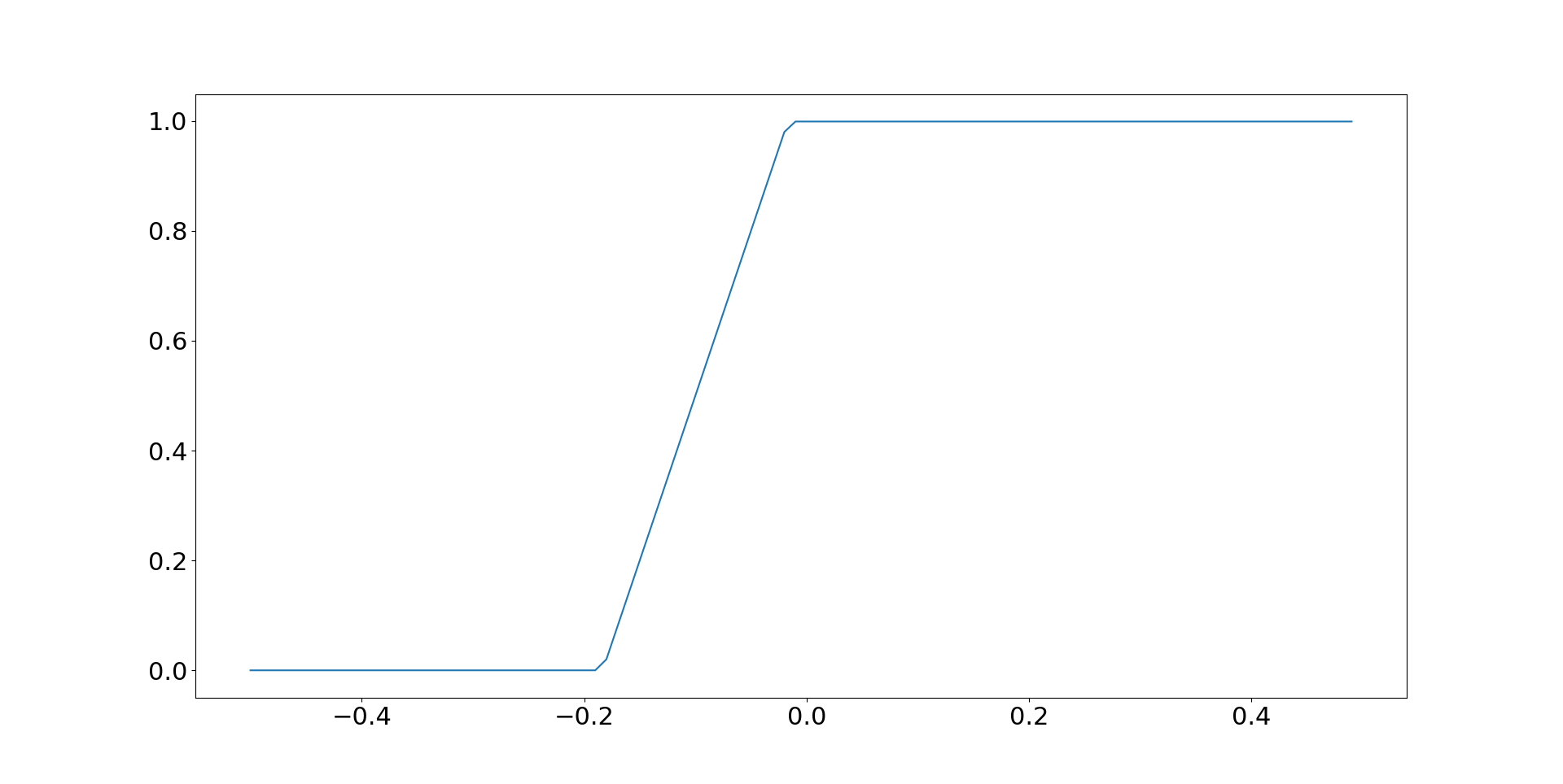
Now, what about the effects of dynamic optimisation. Because dynamic optimisation only makes sense across instruments, I'm going to do this exercise for 50 or so randomly selected instruments (50 rather than 200 to save time running backtests - it won't affect the results much). 

The y-axis shows the turnover, with each line representing a different trading speed.

The x-axis labels are as follows:

• The total turnover of the strategy before any dynamic optimisation takes place; this is analogous to the raw position in the table above. Again this is higher than the figures for the S&P 500 above because of the effect of instrument diversification.
• The total turnover of the strategy after dynamic optimisation, but without any cost penalty or buffering.
• The total turnover of the strategy after dynamic optimisation, with a cost penalty, but with no buffering.
• The total turnover of the strategy after dynamic optimisation, without a cost penalty, but with buffering.
• The total turnover of the strategy after dynamic optimisation, with a cost penalty and buffering.

Interestingly the optimisation adds a 'fixed cost' of turnover to the strategy of extra turnover per year, although this does not happen with the fastest rule. Both buffering and the trading cost penalty reduce the turnover, although the cost penalty has the larger standalone effect. Taken together, costs and buffering reduce turnover significantly, between around a half and a third.

What does this all mean? Well it means we probably have a little more headroom than we think when considering whether a particular trading rule is viable, since it's likely the net effect of position sizing plus buffering will slow things down. This isn't true for the very slowest trading rules with dynamic optimisation which can't quite overcome the turnover increase from position sizing, but they this is unlikely to be an issue for the cheaper instruments where we'd consider adding a faster trading rule.

Changes in costs (dynamic optimisation)

You might expect higher turnover to always linearly lead to higher costs. That's certainly the case for the simple one instrument, S&P 500 only, setup above. But this is not automatically the case for dynamic optimisation. Indeed, we can think of some pathological examples where the turnover is much higher for a given strategy, but costs are lower, because the DO has chosen to trade instrument(s) with lower costs.

In fact the picture here is quite similar to turnover, so the point still stands. We can knock off about 1/3 of the costs of trading the very fastest EWMA through the use of dynamic optimisation with a cost penalty (and buffering also helps). Even with the slowest of our EWMA we still see a 25% reduction in costs.  

Forecast combination

Now let us move from a simple world in which we are selecting a single momentum rule, and foolishly trading it on every instrument we own regardless of costs, to one in which we trade multiple momentum rules.

There is another effect at work in a full fledged trading strategy, that won't be obvious from the isolated research we've done so far, and that is forecast combination. If we introduce a new fast trading rule, we're unlikely to give it 100% of the forecast weights. This means that it's effect on the overall turnover of the strategy will be limited.

To take a simple example, suppose we're trading a strategy with a forecast turnover of 15, leading to a likely final turnover of ~13.3 after buffering and what not (as explained above). Now we introduce a new trading rule with a 10% allocation, that has a turnover of 25. If the trading rule has zero correlation with the other rules, then our forecast turnover will increase to (0.9 * 15) + (0.1 * 25) = 16. After buffering and what not the final turnover will be around 14.0. A very modest increase really.

This is too simplified. If a forecast really is uncorrelated, then it adding it will increase the forecast diversification multiplier (FDM), which will increase the turnover of the final combined forecast. But if the forecast is highly correlated, then the raw turnover will increase by more than we expect. In both of these cases get slightly more turnover; so things will be a little worse than we expect.

Implications for the speed limit

A reminder: I have a trading speed limit concept which states that I don't want to allocate more than third of my expected pre-cost Sharpe Ratio towards trading costs. For an individual trading rule on a single instrument, that equates to a maximum of around 0.13 or 0.10 SR annual units to be spent on costs, depending on which of my books you are reading (consistency is for the hoi polloi).  The logic is that the realistic median performance for an individual instrument is unlikely to be more than 0.40 or 0.30 SR.

(At a portfolio level we get higher costs because of additional leverage from the instrument diversification multiplier, but as long as the realised improvement in Sharpe Ratio is at least as good as that we'll end up paying the same or a lower proportion in expected costs).

How does that calculation work in practice? Suppose you are trading an instrument which rolls quarterly, and you have a cost of 0.005 SR units per trade. The maximum turnover for a forecast to meet my speed limit, and thus be included in the forecast combination for a given instrument, assuming a speed limit of 0.13 SR units is:

Annual cost, SR units = (forecast turnover + rolls per year) * cost per trade 

Maximum annual cost, SR units = (maximum forecast turnover + rolls per year) * cost per trade 

Maximum forecast turnover = (Maximum annual cost / cost per trade) - rolls per year

Maximum forecast turnover = (0.13 / 0.005) - 4 = 22

However that ignores the effect of everything we've discussed so far:

• forecast combination 
• the FDM (adds leverage, makes things worse)
• other sources of position turnover, mainly vol scaling (makes things better for very fast rules)
• the IDM multiplier (adds leverage, makes things worse)
• buffering (static system) - makes things better
• buffering and cost penalty (DO) - makes things better

Of course it's better, all other things being equal, to trade more slowly and spend less on costs but all of this suggests we probably do have room to make a modest allocation to a relatively fast trading rule without it absolutely killing us on trading costs.

An experiment with combined forecasts

Let's setup the following experiment. I'm interested in three different setups:

1. Allocating only to the very slowest three momentum speed (regardless of instrument cost, equally weighted)
2. Allocating only to the very fastest three momentum speeds (regardless of instrument cost, equally weighted)
3. Allocating conditionally to momentum speeds depending on the costs of an instrument and the turnover of the trading rule, ensuring I remain below the 'speed limit'. This is what I do now. Note that this will imply that some instruments are excluded.
4. Allocating to all six momentum speeds in every instrument (regardless of instrument cost, equally weighted)

1. is a fast system, whilst 2. is a 'slow' system (it's not that slow!). In the absence of costs, we would probably want to trade them both, given the likely diversification and other benefits. Options 3 and 4 explore two different ways of doing that. Option 3 involves throwing away trading rules that are too quick for a given instrument, whilst option 4 ploughs on hoping everything will be okay.

How should we evaluate these? Naturally, we're probably most interested in the turnover and costs of options 3 and 4. It will be interesting to see if the costs of option 4 are a hell of a lot higher, or if we are managing to 'smuggle in'.

What about performance? Pure Sharpe ratio is one way, but may give us a mixed picture. In particular, the pre-cost SR of the faster rules has historically been worse than the slower rules. The fourth option will produce a 50:50 split between the two, which is likely to be sub-optimal. Really what we are interested in here is the 'character' of the strategies. Hence a better way is to run regressions of 3 and 4 versus 1 and 2. This will tell us the implicit proportion of fast trading that has survived the various layers between forecast and position.

Nerdy note: Correlations between 1 and 2 are likely to be reasonably high (around 0.80), but not enough to cause problems with co-linearity in the regression.

To do this exercise I'm going to shift to a series of slightly different portfolio setups. Firstly, I will use the full 102 instruments in my 'jumbo portfolio'. Each of these has met a cutoff for SR costs per transaction. I will see how this does for both the static set of instruments (using a notional $50 million to avoid rounding errors), but also for the dynamic optimisation (using $500K). 

However I'm also going to run my full list of 176 instruments only for dynamic optimisation, which will include many instruments that are far too expensive to meet my SR cost cutoff or are otherwise too illiquid (you can see a list of them in this report; there are about 70 or so at the time of writing; there is no point doing this for static optimisation as the costs would be absolutely penal for option 4). I will consider two sub options here: forming forecasts for these instruments but not trading them (which is my current approach), and allowing them to trade (if they can survive the cost penalty, which I will still be applying).

Note that I'm going to fit instrument weights (naturally in a robust, 'handcrafted' setup using only correlations). Otherwise I'd have an unbalanced portfolio, since there are more equities in my data set than other instruments.

To summarise then we have the following four scenarios in which to test the four options:

1. Static system with 102 instruments ($50 million capital)
2. Dynamic optimisation with 102 instruments ($500k)
3. Dynamic optimisation with 176 instruments, constraining around 70 expensive or illiquid instruments from trading ($500k)
4. Dynamic optimisation with 176 instruments, allowing expensive instruments to trade (but still applying a cost penalty) ($500k)

Results

Let's begin as before by looking at the total turnover and costs. Each line on the graph shows a different scenario:

1. (Static) Static system with 102 instruments ($50 million capital)
2. (DO_cheap) Dynamic optimisation with 102 instruments ($500k), which excludes expensive and illiquid instruments
3. (DO_constrain) Dynamic optimisation with 176 instruments, constraining around 70 expensive or illiquid instruments from trading ($500k)
4. (DO_unconstrain) Dynamic optimisation with 176 instruments, allowing expensive instruments to trade (but still applying a cost penalty) ($500k)

 The x-axis show the different options: 

1. (slow) Allocating only to the very slowest three momentum speed (regardless of instrument cost, equally weighted)
2. (fast) Allocating only to the very fastest three momentum speeds (regardless of instrument cost, equally weighted)
3. (condition) Allocating conditionally to momentum speeds depending on the costs of an instrument and the turnover of the trading rule, ensuring I remain below the 'speed limit'. This is what I do now. Note that this will imply that some instruments are excluded completely.
4. (all) Allocating to all six momentum speeds in every instrument (regardless of instrument cost, equally weighted)

First the turnovers

Now the costs (in SR units):

These show a similar pattern, but the difference between lines is more marked for costs. Generally speaking the static system is the most expensive way to trade anything. This is despite the fact that it does not have any super expensive instruments, since these have already been weeded out. Introducing DO with a full set of instruments, including many that are too expensive to trade, and allowing all of them to trade still reduces costs by around 20% when trading the three fastest rules or all six rules together.

Preventing the expensive instruments from trading (DO_constrain) lowers the costs even further, by around 30% [Reminder: This is what I currently do]. Completely removing expensive instruments provides a further reduction, but it is negligible.

Conditionally trading fast rules, as I do now, allows us to trade pretty much at the same cost level as a slow system: it's only 1 basis point of SR more expensive. But trading all trading rules for all instruments is a little more pricey. 

Now how about considering the 'character' of returns? For each of the options 3 and 4, I am going to regress their returns on the returns of option 1 and option 2. The following tables shows the results. Each row is a scenario, and the columns show the betas on 'slow' (option 1) and 'slow' respectively. I've resampled returns to a monthly frequency to reduce the noise.

First let's regress the returns from a strategy that uses *all* the trading rules for every instrument.

                 fast   slow
static          0.590  0.557
DO_cheap        0.564  0.557
DO_constrain    0.550  0.561
DO_unconstrain  0.535  0.559

Each individual instrument is 50% fast, 50% slow, so this is exactly what we would expect with about half the returns of the combined strategy coming from exposure to the fast strategy, and about half from the slow (note there is no constraint for the Betas to add up to one, and no reason why they would do so exactly).

Now let's regress the returns from a conditional strategy on the fast and slow strategies in each scenario:

                fast   slow
static          0.762  0.337
DO_cheap        0.743  0.313
DO_constrain    0.805  0.288
DO_unconstrain  0.786  0.271

This is.... surprising! About 75% of the returns of the conditional strategy come from exposure to the fast trading rules, and 25% from the slow ones. By only letting the cheapest instruments trade the fast strategy, we've actually made the overall strategy look more like a fast strategy. 

Conclusions

This has been a long post! Let me briefly summarise the implications.

• Buffering in a static system reduces turnover, and thus costs, by 17% on a very fast strategy giving us a little more headroom on the 'speed limit' that we think we have.
• Dynamic optimisation has the same effect, but is more efficient reducing costs by around a third; as unlike static buffering the cost penalty is instrument specific.
• It's worth preventing expensive instruments from trading in DO, as the cost penalty doesn't seem to be 100% efficient in preventing them from trading. But there isn't any benefit in completely excluding these expensive instruments from the forecast construction stage.
• Surprisingly, allowing expensive instruments to trade quicker trading rules actually makes a strategy less correlated to a faster trading strategy. It also increases costs by around 50% versus the conditional approach (where only cheap instruments can trade quick rules). 

Good news: all of this is a confirmation that what I'm currently doing* is probably pretty optimal! 

* running DO with expensive instruments, but not allowing them to trade, and preventing expensive instruments from using quicker trading rules.

Bad news: it does seem that my original idea of just trading more fast momentum, in the hope of 'smuggling in' some more diversifying trading rules, is a little dead in the water.

In the next post, I will consider an alternative way of 'smuggling in' faster trading strategies - by using them as an execution overlay on a slower system.