This is a short follow up post to one I did a couple of years ago, on "Exogenous risk management". This was quite an interesting post which dug into why expected risk changes for a typical diversified futures trading system. And then I introduced my risk overlay:
"Now we have a better understanding of what is driving our expected risk, it's time to introduce the risk overlay. The risk overlay calculates a risk position multiplier, which is between 0 and 1. When this multiplier is one we make no changes to the positions calculated by our system. If it was 0.5, then we'd reduce our positions by half. And so on.
Since I wrote that post, I've radically changed the way my trading strategy is designed. This is discussed at length here. Here are some relevant highlights
- ....
- A risk overlay (actually was in my old system, but not yet in my new system - a change I plan to make soon)
- ....
- Dynamic optimisation using minimum tracking error (here and here)
- .....
- Estimating vol using a partially mean reverting method
Basically I did a lot of stuff, but along the way I lost my risk overlay. But like I said above, I planned to reintroduce it once the dust had settled. Can you hear that noise? That's sound the sound of dust settling. Also note that I introduced a new method for estimating vol. That will be important later.
There will be some very specific references to my open source trading system pysystemtrade, but the vast majority of this post should be of general interest to most people who are interested in risk management.
Where should the risk overlay go?
This was a question that wasn't an issue before, but now I have my new fancy dynamic optimisation method, where should the risk overlay go? Should it go into the upstream methodology that calculates an optimal unrounded set of positions? Or should it go into the actual dynamic optimisation itself? Or should it go into a downstream process that runs after the dynamic optimisation?
On reflection I decided not to put the overlay into the dynamic optimisation. You can imagine how this would have worked; we would have added the risk limits as additional constraints on our optimisation, rather than just multipling every positions by some factor betwen 0 and 1. It's a nice idea, and if I was doing a full blown optimisation it would make sense. But I'm using a 'greedy algo' for my optimisation, which doesn't exhaustively search the available space. That makes it unsuitable for risk based constraints.
I also decided not to put the overlay into a downstream process. This was for a couple of reasons. Firstly, in production trading the dynamic optimisation is done seperately from the backtest, using the actual live production database to source current positions and position constraint + trade/no-trade information. I don't really want to add yet more logic to the post backtest trade generation process. Secondly - and more seriously - having gone to a lot of effort to get the optimal integer positions, applying a multiplier to these would most probably result in a lot of rounding going on, and the resulting set of contract positions would be far from optimal.
This leaves us with an upstream process; something that will change the value of system.portfolio.get_notional_positions(instrument_code) - my optimal unrounded positions.
What risks am I concerned about?
Rather than just do a wholesale implementation of the old risk overlay, I thought it would be worthwhile considering from scratch what risks I am concerned about, and whether the original approach is the best way to avoid them.
- Expected risk being just too high. In the original risk overlay, I just calculated expected risk based on estimated correlations and standard deviations.
- The risk that volatility will jump up. Specifically, the risk that it will jump to an extreme level. This risk was dealt with in the risk overlay by recalculating the expected risk, but replacing the current standard deviation with the '99' standard deviation: where % standard deviation would be for each instrument at the 99% percentile of it's distribution.
- The risk that vol is too low compared to historic levels. I dealt with this previously in the 'endogenous' risk management eg within the system itself not the risk overlay, by not allowing a vol estimate to go below the 5% percentile of it's historic range.
- A shock to correlations. For example, if we have positions on that look they are hedging, but correlations change to extreme values. This risk was dealt with in the risk overlay by recalculating the expected risk with a correlation matrix of +1,-1; whatever is worse.
Here is what I decided to go with:
- Expected risk too high: I will use the original risk overlay method
- Vol jump risk: I will use the original method, the '99' standard deviation.
- Vol too low risk: I have slready modified my vol estimate, as I noted above, so that it's a blend of historic and current vol. This removes the need for a percentile vol floor.
- Correlation shock: I replaced with the equivalent calculation, a limit on sum(abs(annualised risk % each position)). This is quicker to calculate and more intuitive, but it's the same measure. Incidentally, capping the sum of absolute forecast values weighted by instrument weights would achieve a similar result, but I didn't want to use forecasts, to allow for this method being universal across different types of trading strategy.
- Leverage risk (new): The risk of having positions whose notional exposure is an unreasonable amount of my capital. I deal with this by using specific position limits on individual instruments.
- Leverage risk 2 (new): The implication of a leverage limit is that there is a minimum % annualised risk we can have for a specific instrument. I deal with this by removing instruments whose risk is too low
- Leverage risk 3: At an aggregate level in the risk overlay I also set a limit on sum(abs(notional exposure % each position)). Basically this is a crude leverage limit. So if I have $1,000,000 in notional positions, and $100,000 in capital, this would be 10.
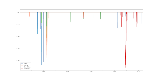
Hence we have the following risk control measures:
- Endogenous
- Risk overlay
- Normal: Estimated risk limit
- Jump: Estimated risk with 99% vol
- Correlation: Sum(abs(% annualised risk each position))
- Leverage: Sum(abs(notional exposure % each position))
- Off-line
- Specific position limits to avoid any given instrument having a notional position that is too hight
- Instrument selection to avoid instruments whose % risk is too low
Off line
Let's being by quickly talking about the 'off-line' risk controls: specific position limits, and minimum standard deviation.
Firstly, we only select instruments to trade that have some minimum standard deviation.
It can be shown (see my forthcoming book for proof!) that there is a lower limit on the instrument risk (s), given a maximum resulting leverage ratio (size of notional position in that instrument divided by total capital) L, instrument weight w, annualised risk target (t), and instrument diversification multiplier (IDM). Assuming the ratio of maximum forecast to average forecast is 2:
Minimum s = (2 × IDM × w × t) ÷ L
For example, if the instrument weight is 1%, the IDM is 2.5, the risk target is 25%, and we don't want more than 100% of our notional in a specific instrument (L=1) then the minimum standard deviation is 2 * 2.5 * 0.01 * 0.25 / 1 = 1.25%.
That's pretty low, but it would sweep up some short duration bonds. Here's the safest instruments in my data set right now:
EURIBOR         0.287279 *
SHATZ           0.553181 *
US2             0.791563 *
EDOLLAR         0.801186 *
JGB             1.143264 *
JGB-SGX-mini    1.242098 *
US3             1.423352
BTP3            1.622906
KR3             1.682838
BOBL            2.146153
CNH-onshore     2.490476
It looks like those marked with * ought to be excluded from trading. Incidentally, the Shatz and JGB mini are already excluded on the grounds of costs.
This will affect the main backtest, since we'll eithier remove such instruments entirely, or - more likely - mark them as 'bad markets' which means I come up with optimal positions for them, but then don't actually allow the dynamic optimisation to utilise them.
Note that it's still possible for instruments to exceed the leverage limit, but this is dealt with by the off line hard position limits. Again, from my forthcoming book:
Maximum N = L × Capital ÷ Notional exposure per contract
Suppose for example we have capital of $100,000; and a notional exposure per contract of $10,000. We don’t want a leverage ratio above 1. This implies that our maximum position limit would be 10 contracts.
We can check this is consistent with the minimum percentage risk imposed in the example above with a 1% instrument weight, IDM of 2.5, and 25% risk target. The number of contracts we would hold if volatility was 1.25% would be (again, formula from my latest book although hopefully familar):
Ni = (Forecast ÷ 10) × Capital × IDM × weighti × t ÷
(Notional exposure per contract × s%, i)
= (20 ÷ 10) × 100000 × 2.5 × 0.01 × 0.25 ÷ (10,000 ×0.0125)
= 10 contracts
Because the limits depend on the notional size of each contract they ought to be updated regularly. I have code that calculates them automatically, and sets them in my database. The limits are used in the dynamic optimisation; plus I have other code that ensures they aren't exceeded by blocking trades which would otherwise cause positions to increase.
Note: These limits are not included in the main backtest code, and only affect production positions. It's possible in theory to test the effect of imposing these constraints in a backtest, but we'd need to allow these to be historically scaled. This isn't impossible, but it's a lot of code to write for little benefit.
Risk overlay
Once we've decided what to measure, we need to measure it, before we decide what limits to impose.
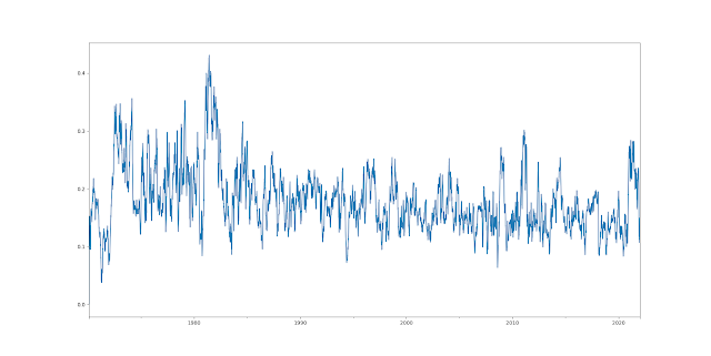
- Normal: Estimated risk limit
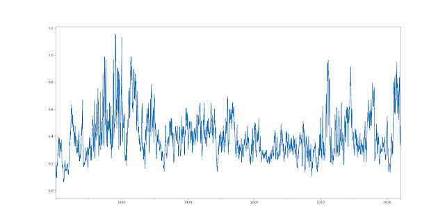
- Jump: Estimated risk with 99% vol
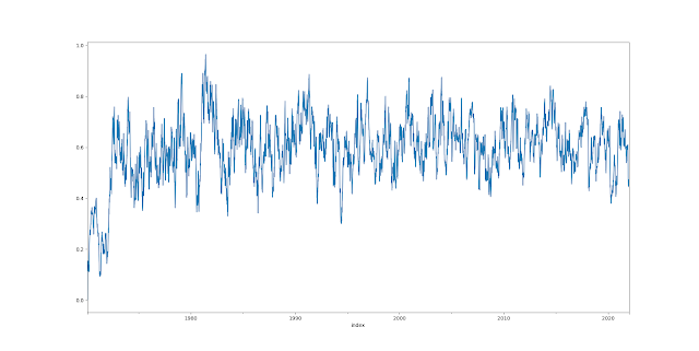
- Correlation: Sum(abs(% annualised risk each position))
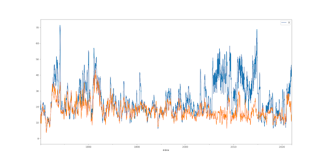
- Leverage: Sum(abs(notional exposure % each position))
risk_overlay:
  max_risk_fraction_normal_risk: 1.4
  max_risk_fraction_stdev_risk: 3.6
  max_risk_limit_sum_abs_risk: 3.4
  max_risk_leverage: 13.0
Summary
That's probably it in terms of modifying my flagship system for a while - probably a good thing after quite a few changes in a relatively short time!
Hi Rob,
ReplyDeleteRegarding 'normal' risk, the target was 25% but the median came in at 16.9%, which was attributed to the IDM not allowing some instrument leverage. It seems you have since increased the IDM to 2.75 (or more). I was wondering if this could alternatively be attributed to individual instrument position limits, and if so, is there a concern that this will lead to an undershoot of the risk target over time?
I think I know your answer to the next question, but have to ask - if there is a downward bias from the targeted portfolio level risk, would you ever increase the target, from say 25% to 30%, in order to achieve the 25% target?
Thanks,
Yes I've increased the IDM because the correlation matrix underestimates the degree of diversification so expected risk is lower than target which makes me more relaxed. "if there is a downward bias from the targeted portfolio level risk, would you ever increase the target, from say 25% to 30%, in order to achieve the 25% target?" No, and I've actually undershot quite consistently in live trading and this doesn't bother me.
Delete