Optimal trend following allocation under conditions of uncertainty and without secular trends

Few people are brave enough to put their entire net worth into a CTA fund or home grown trend following strategy (my fellow co-host on the TTU podcast, Jerry Parker, being an honorable exception with his 'Trend following plus nothing' portfolio allocation strategy). Most people have considerably less than 100% - and I include myself firmly in that category. And it's probably true that most people have less than the sort of optimal allocation that is recommended by portfolio optimisation engines.

Still it is a useful exercise to think about just how much we should allocate to trend following, at least in theory. The figure that comes out of such an exercise will serve as both a ceiling (you probably don't want any more than this), and a target (you should be aiming for this). 

However any sort of portfolio optimisation based on historical returns is likely to be deeply flawed. I've covered the problems involved at length before, in particular in my second book and in this blogpost, but here's a quick recap:

1. Standard portfolio optimisation techniques are not very robust
2. We often assume normal distributions, but financial returns are famously abnormal
3. There is uncertainty in the parameter estimates we make from the data
4. Past returns distributions may be biased and unlikely to repeat in the future

As an example of the final effect, consider the historically strong performance of equities and bonds in a 60:40 style portfolio during my own lifetime, at least until 2022. Do we expect such a performance to be repeated? Given it was driven by a secular fall in inflation from high double digits, and a resulting fall in interest rates and equity discount rates, probably not. 

Importantly, a regime change to lower bond and equity returns will have varying impact on a 60:40 long only portfolio (which will get hammered), a slow trend following strategy (which will suffer a little), and a fast trend following strategy (which will hardly be affected). 

Consider also the second issue: non Gaussian return distributions. In particular equities have famously negative skew, whilst trend following - especially the speedier variation - is somewhat positive in this respect. Since skew affects optimal leverage, we can potentially 'eat' extra skew in the form of higher leverage and returns. 

In conclusion then, some of the problems of portfolio optimisation are likely to be especially toxic when we're looking at blends of standard long only assets combined with trend following. In this post I'll consider some tricks methods we can use to alleviate these problems, and thus come up with a sensible suggestion for allocating to trend following. 

If nothing else, this is a nice toy model for considering the issues we have when optimising, something I've written about at length eg here. So even if you don't care about this problem, you'll find some interesting ways to think about robust portfolio optimisation within.

Credit: This post was inspired by this tweet.

Some very messy code with hardcoding galore, is here.

The assets

Let's first consider the assets we have at our disposal. I'm going to make this a very simple setup so we can focus on what is important whilst still learning some interesting lessons. For reasons that will become apparent later, I'm limiting myself to 3 assets. We have to decide how much to allocate to each of the following three assets:

• A 60:40 long only portfolio of bonds and equities, represented by the US 10 year and S&P 500
• A slow/medium speed trend following strategy, trading the US 10 year and S&P 500 future with equal risk allocation, with a 12% equity-like annualised risk target. This is a combination of EWMAC crossovers: 32,128 and 64,256
• A relatively fast trend following strategy, trading the US 10 year and S&P 500 future with equal risk allocation, with a 12% annualised risk target. Again this is a combination of EWMAC crossovers: 8, 32 and 16,64

Now there is a lot to argue with here. I've already explained why I want to allocate seperately to fast and slow trend following; as it will highlight the effect of secular trends.

The reason for the relatively low standard deviation target is that I'm going to use a non risk adjusted measure of returns, and if I used a more typical CTA style risk (25%) it would produce results that are harder to interpret.

You may also ask why I don't have any commodities in my trend following fund. But what I find especially interesting here is the effect on correlations between these kinds of strategies when we adjust for long term secular trends. These correlations will be dampened if there are other instruments in the pot. The implication of this is that the allocation to a properly diversified trend following fund running futures across multiple asset classes will likely be higher than what is shown here.

Why 60:40? Rather than 60:40, I could directly try and work out the optimal allocation to a universe of bonds and equities seperately. But I'm taking this as exogenous, just to simplify things. Since I'm going to demean equity and bond returns in a similar way, this shouldn't affect their relative weightings.

50:50 risk weights on the mini trend following strategies is more defensible; again I'm using fixed weights here to make things easier and more interpretable. For what it's worth the allocation within trend following for an in sample backtest would be higher for bonds than for equities, and this is especially true for the faster trading strategy.

Ultimately three assets makes the problem both tractable and intuitive to solve, whilst giving us plenty of insight.

Characteristics of the underyling data

Note I am going to use futures data even for my 60:40, which means all the returns I'm using are excess returns.

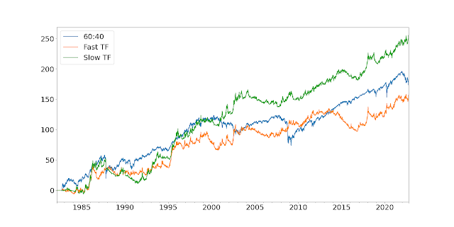
Let's start with a nice picture:

So the first thing to note is that the vol of the 60:40 is fairly low at around 12%; as you'd expect given it has a chunky allocation to bonds (vol ~6.4%). In particular, check out the beautifully smooth run from 2009 to 2022. The two trading strategies also come in around the 12% annualised vol mark, by design. In terms of Sharpe Ratio, the relative figures are 0.31 (fast trading strategy), 0.38 (long only) and 0.49 (slow trading strategy). However as I've already noted, the performance of the long only and slow strategies is likely to be flattered by the secular trends in equities and bonds seen since 1982 (when the backtest starts).

Correlations matter, so here they are:

         60:40  Fast TF  Slow TF
60:40     1.00    -0.02     0.25
Fast TF  -0.02     1.00     0.68
Slow TF   0.25     0.68     1.00

What about higher moments? The monthly skews are -1.44 (long only), 0.08 (slow) and 0.80 (fast). Finally what about the tails? I have a novel method for measuring these which I discuss in my new book, but all you need to know is that a figure greater than one indicates a non-normal distribution. The lower tail ratios are 1.26 (fast), 1.35 (slow) and 2.04 (long only); whilst the uppers are 1.91 (fast), 1.74 (slow) and 1.53 (long only). In other words, the long only strategy has nastier skew and worst tails than the fast trading strategy, whilst the slow strategy comes somewhere in between.

Demeaning

To reiterate, again, the performance of the long only and slow strategies is likely to be flattered by the secular trends in equities and bonds, caused by valuation rerating in equities and falling interest rates in bonds. 

Lets take equities. The P/E ratio in September 1982 was around 9.0, versus 20.1 now. This equates to 2.0% a year in returns coming from the rerating of equities. Over the same period US 10 year bond yields have fallen from around 10.2% to 4.0% now, equating to around 1.2% a year in returns. I can do a simple demeaning to reduce the returns achieved by the appropriate amounts.

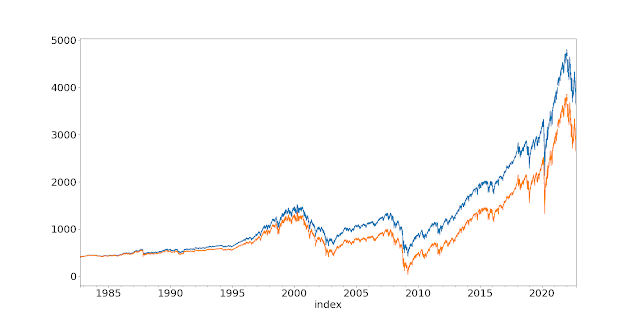
Here are the demeaned series with the original backadjusted prices. First S&P:

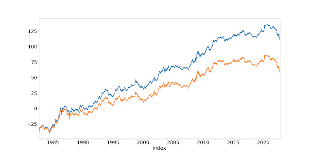
And for US10:

What effect does the demeaning have? It doesn't affect significantly standard deviations, skew, or tail ratios. But it does affect the Sharpe Ratio:

              Original       Demean     Difference

Long only       0.38          0.24        -0.14

Slow TF         0.49          0.41        -0.08

Fast TF         0.31          0.25        -0.06

This is exactly what we would expect. The demeaning has a larger effect on the long only 60:40, and to a lesser extent the slower trend following. 

And the correlation is also a little different:

         60:40  Fast TF  Slow TF
60:40     1.00    -0.06     0.18
Fast TF  -0.06     1.00     0.66
Slow TF   0.18     0.66     1.00

Both types of trend have become slightly less correlated with 60:40, which makes sense.

The optimisation

Any optimisation requires (a) a utility or fitness function that we are maximising, and (b) a method for finding the highest value of that function. In terms of (b) we should bear in mind the comments I made earlier about robustness, but let's first think about (a).

An important question here is whether we should be targeting a risk adjusted measure like Sharpe Ratio, and hence assuming leverage is freely available, which is what I normally do. But for an exercise like this a more appropriate utility function will target outright return and assume we can't access leverage. Hence our portfolio weights will need to sum to exactly 100% (we don't force this to allow for the possibility of holding cash; though this is unlikely). 

It's more correct to use geometric return, also known as CAGR, rather than arithmetic mean since that is effectively the same as maximising the (log) final value of your portfolio (Kelly criteria). Using geometric mean also means that negative skew and high kurtosis strategies will be punished, as will excessive standard deviation. By assuming a CAGR maximiser, I don't need to worry about the efficient frontier, I can maximise for a single point. It's for this reason that I've created TF strategies with similar vol to 60:40.

I'll deal with uncertainty by using a resampling technique. Basically, I randomly sample with replacement from the joint distribution of daily returns for the three assets I'm optimising for, to create a new set of account curves (this will preserve correlations, but not autocorrelations. This would be problematic if I was using drawdown statistics, but I'm not). For a given set of instrument weights, I then measure the utility statistic (CAGR) for the resampled returns. I repeat this exercise a few times, and then I end up with a distribution of CAGR for a given set of weights. This allows us to take into account the effect of uncertainty. 

Finally we have the choice of optimisation technique. Given we have just three weights to play with, and only two degrees of freedom, it doesn't seem too heroic to use a simple grid search. So let's do that.

Some pretty pictures

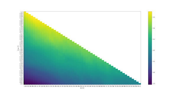
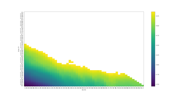
Because we only have two degrees of freedom, we can plot the results on a 2-d heatmap. Here's the results for the median CAGR, with the original set of returns before demeaning:

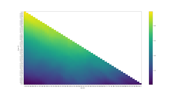
Sorry for the illegible labels - you might have to click on the plots to see them. The colour shown reflects the CAGR. The x-axis is the weight for the long only 60:40 portfolio, and the y-axis for slow trend following. The weight to fast trend following will be whatever is left over. The top diagonal isn't populated since that would require weights greater than 1; the diagonal line from top left to bottom right is where there is zero weight to fast trend following; top left is 100% slow TF and bottom right is 100% long only.

Ignoring uncertainty then, the optimal weight (brightest yellow) is 94% in slow TF and 6% in long only. More than most people have! However note that there is a fairly large range of yellow CAGR that are quite similar. 

The 30% quantile estimate for the optimal weights is a CAGR of 4.36, and for the 70% quantile it's 6.61. Let's say we'd be indifferent between any weights whose median CAGR falls in that range (in practice then, anything whose median CAGR is greater than 4.36). If I replace everything that is statistically indistinguishable from the maximum with white space, and redo the heatmap I get this:

This means that, for example, a weight of 30% in long only, 34% in slow trend following, and 36% in fast trend following; is just inside the whitespace and thus is statistically indistinguishable from the optimal set of weights. Perhaps of more interest, the maximum weight we can have to long only and still remain within this region (at the bottom left, just before the diagonal line reappears) is about 80%.

Implication: We should have at least 20% in trend following.

If I had to choose an optimal weight, I'd go for the centroid of the convex hull of the whitespace. I can't be bothered to code that up, but by eye it's at roughly 40% 60/40, 50% slow TF, 10% fast TF.

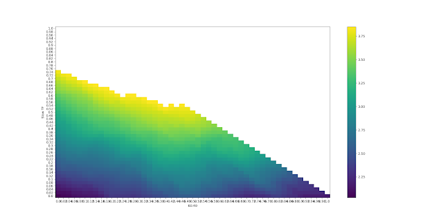
Now let's repeat this exercise with the secular trends removed from the data.

The plot is similar, but notice that the top left has got much better than the bottom right; we should have a lower weight to 60:40 than in the past. In fact the optimal is 100% in slow trend following; zilch, nil, zero, nada in both fast TF and 60:40.

But let's repeat the whitespace exercise to see how robust this result is:

The whitespace region is much smaller than before, and is heavily biased towards the top left. Valid portfolio weights that are indistinguishable from the maximum include 45% in 60:40 and 55% in slow TF (and 45% is the most you should have in 60:40 whilst remaining in this region). We've seen a shift away from long only (which we'd expect), but interestingly no shift towards fast TF, which we might have expected as it is less affected by demeaning.

The optimal (centroid, convex hull, yada yada...) is somewhere around 20% 60:40, 75% slow TF and 5% in fast TF.

Summary: practical implications

This has been a highly stylised exercise, deliberately designed to shine a light on some interesting facts and show you some interesting ways to visualise the uncertainty in portfolio optimisation. You've hopefully seen how we need to consider uncertainty in optimisation, and I've shown you a nice intuitive way to produce robust weights.

The bottom line then is that a robust set of allocations would be something like 40% 60/40, 50% slow TF, 10% fast TF; but with a maximum allocation to 60/40 of about 80%. If we use data that has had past secular trends removed, we're looking at an even higher allocation to TF, with the maximum 60/40 allocation reducing considerably, to around 45%. 

Importantly, this has of course been an entirely in sample exercise. Although we've made an effort to make things more realistic by demeaning, much of the results depend on the finding that slow TF has a higher SR than 60:40, an advantage that is increased by demeaning. Correcting for this would result in a higher weight to 60:40, but also to fast TF.

Of course if we make this exercise more realistic, it will change these results:

• Improving 60:40 equities- Introducing non US assets, and allocating to individual equities
• Improving 60:40 bonds -  including more of the term structure, inflation and corporate bonds, 
• Improving 60:40 by including other non TF alternatives
• Improving the CTA offering - introducing a wider set of instruments across asset classes (there would also be a modest benefit from widening beyond a single type of trading rule)
• Adding fees to the CTA offering 

I'd expect the net effect of these changes to result in a higher weight to TF, as the diversification benefits in going from two instruments to say 100 is considerable; and far outweights the effect of fees and improved diversification in the long only space.

The three kinds of (over) fitting

This post is something that I've banged on about in many presentations at several conferences* (most complete slides are here), and in various interviews, but never actually formally described in a blog post. In fact this post has existed in draft form since 2015 (!).

* you know, when you leave your house and listen to someone else speaking. Something that in late 2021 is a distant memory, although I will actually be speaking at an event later this year.

So there won't be new information here if you've been following my work closely, but it's still nice to write it down in one place.

(I'm trying to stick to my self imposed target of one blog post per month, but you will appreciate that I don't always have time for the research involved in producing them - unless it's a by product of something I'm already working on)

Trivially, it's about the fitting of trading systems and the different ways you can screw this up:

• Explicit (over)fitting
• Implicit (over)fitting
• Tacit (over)fitting

What is fitting

I find it hard to believe that anyone reading this doesn't already know this, unless you've accidentally landed here after googling some unrelated search term, but let me define my terms.

The act of fitting a trading system can formally be defined as the process of discovering which combination of trading rule and parameter set(s) will produce the optimal trading system when tested on historic data: a combination I call the trading rule variation. The unspoken assumption of all quant finance is that this variation will also be the optimal system to use in the future.

A trading rule is a specific set of instructions which tells you how to trade; for example something like 'Buy if the N day return is negative, otherwise sell'. In this case the parameter set would consist only of a specific value of N.

Optimality can mean many things, but for the purposes of this post let's assume it's maximising Sharpe Ratio (it isn't that important which measure we choose in the context of our discussion here).

So for this particular example fitting could involve considering alternative values of N, and finding the value which had the highest Sharpe Ratio in an historic backtest. Alternatively, it could also involve trying out different rules - for example 'Sell if the N day return is negative, otherwise buy'. But note that these approaches are equivalent; we could parameterize this alternative set of rules as 'Buy X*units if the N day return is negative, otherwise buy' where X is eithier +1 (so we buy) or -1 (so we sell). Now we have two parameters, N and X, and our fitting process will try and find the optimal joint parameter values. 

Of course there are still numerous rules that we haven't considered here, such as selling if the N hour return is negative, or if the most recent non farm payroll was greater than N, or if there was a vomiting camel chart pattern on the Nth Wednesday in the month. So when fitting we will do so over a given parameter space, which includes the range of possible values for all our parameters. Here the parameter space will be X = [-1,1] and N = [1,2,3......] (assuming we have daily closing data). The product of possible values of X and N can loosely be thought of as the 'degrees of freedom' of the fitting process. 

All fitting thus involves the choice of some possible trading strategies from a tiny subset of all possible strategies.

The number of units to buy or sell is another question entirely, which I discuss in this series of posts

Fitting can be done in an automated fashion, purely manually, or using some combination of the above. For example, we could get some backtesting software and ask it to find the optimal values of X and N. Or we could manually test each possible variation. Or we could run the backtesting software once for X=1 (buy if N day return is negative), and then again for X=-1, each time finding the best value of N. The third option is the more common amongst most quant traders.

What is overfitting and why it be bad

Consider the following:

Hastie et al (2009) “The Elements of Statistical Learning” Springer. Figure 2.11

How does this relate to the fitting of trading systems? Well, we can think of 'prediction error' as 'Sharpe Ratio on an inverted scale' such that a low value is good. And 'model complexity' is effectively the degrees of freedom of the trading strategy.

What is the graph telling us? Well first consider the 'training sample' - the set of data we used to do the fitting on - the dirty red line. As we add complexity we will get a better performing trading strategy (in expectation). In fact it's possible to create a trading strategy with zero prediction error, and thus infinite Sharpe Ratio, if the degrees of freedom are sufficiently large (in a hand waving way, if the complexity in the strategy is equal to the amount of entropy in the data). 

How? Well consider a trading strategy which has the form 'Buy X*units if it's January', 'Buy X*units if it's February'.... If we fit this on past data it's going to do pretty well. Now let's make it even more complex: 'Buy X* units if it's January 3rd 2015', 'Buy X* units if it's January 4th 2015' .... (where January 3rd 2015 is the first day of our price history). This will perfectly predict every single day in the backtest, and thus have infinite Sharpe Ratio.

(More mathematically, if we fit a sufficiently high degree polynomial to the price data, we can get a perfect fit)

On the out of sample (dirty green) line notice that we always do worse (in expectation) than the red line. That's because we'll never do as well in predicting a different data set to what we have trained / fitted our model on. Also notice that the gap between the red and the green line grows as the model gets more complex. The more closely our model fits the backtest period, the less likely it is that it will be able to predict a novel future. 

This means that the green line has a minimum error (~maximum Sharpe Ratio) where we have the optimal amount of complexity (~degrees of freedom). Anything to the right of this point is overfitting (also known as curve fitting).

Sadly, we don't get paid based on how well we predict the in sample data. We get paid for predicting out of sample performance: for predicting the future. And this is much harder! And the Sharpe Ratios will be lower! 

At least in theory! In practice, if you're an academic then you get paid for publishing papers with nice results: papers that predict the past. If you're working for a quant hedge fund then you may be getting paid for coming up with nice backtests that also predict the past. And even as a humble independent trader, we get a kick out of a nice backtest. So for this reason it's very easy to be drawn towards trying to make the in sample line look as possible: which we'll do by making the model more complicated.

Basically: our incentives make us prone to overfitting and towards confounding the red and the green lines.

Explicit fitting

We're now ready to discuss the three kinds of (over)fitting.

The first is explicit fitting. It's what most people think of as fitting. The basic idea being that you get some kind of automated algo to select the best possible set of parameters. This could be very easy: a grid search for example that just tries every possible strategy variation. Or it could be much more complex: some kind of fancy AI technique like a neural network. 

The good news about explicit fitting is that it's possible to do it properly. By which I mean we can:

 

• Restrict ourselves to fewer degrees of freedom
• Enforce a realistic seperation between in and out of sample data in the backtest (the 'no time machine' rule) 
• Use robust fitting techniques to avoid wandering into the overly complex overfitting end of the figure above.

Of course it's also possible to do explicit fitting badly (and plenty of people do!), but at least it's possible to avoid overfitting if you're careful enough.

Fewer degrees of freedom

Consider a more realistic example of an moving average crossover trading rule (MAC) which can be defined using two parameters A and B: signal = MA_A - MA_B, where MA_x is a moving average with lookback x days, and A<>B. Note that if A<B then this will be a momentum rule, whereas if A>B it will be a mean reversion rule. We assume that A and B can take any values in the range 1 to 256 (where 256 is roughly the number of business days in a year); anything longer than this would be an 'investment' rather than a 'trading' strategy.

If we try and fit all 65,280 possible values of A and B individually for each instrument we trade then we're very likely to overfit. We can reduce our degrees of freedom in various ways:

• Restrict A<B [so just momentum]
• Set B = k.A; fit k first, then fit A  [I do this!]
• Restrict A and B to be in the set {1,2,4,8,16,32, ... 256}  [I do this!]
• Use the same A, B for all instruments in a given asset class [discussed here]
• Use the same A,B for all instruments [perhaps after accounting for costs]

Notice that this effectively involves making fitting decisions outside of the explicit fitting... I discuss this some more later. But for now you can note that it's possible to make these kinds of decisions without using real data at all.

No time machine

By 'no time machine', I mean that a parameter set should only be tested on a period of data if it has been fitted only on data that was available on data that was in the past of the testing period.

So for example if we fit from 2000 - 2020, and then test on the same period, then we're cheating - we couldn't have done this without a time machine. If we fit from 2000-2010, and then test from 2011 - 2020; then that's okay. But if we then do a classic ML technique and subsequently fit from 2011-2020 to test from 2000-2010 then we've cheated.

There are two honest options:

• An expanding window; first we fit using data for 2000 (assuming a year gives us enough data to fit with; if we're doing a robust fit that would be fine) and test that model in the year 2001; then we fit using 2000 and 2001, and test that second model in 2002..... then we fit using 2000 - 2019, and then test in the year 2020.
• A rolling window. Say we want to use a maximum of 10 years to fit our data, then we would proceed initially as for an expanding window until we get to .... we fit using 2000 - 2009 and test in the year 2010, then we fit using 2001 - 2010 and test in the year 2011.... then finally we fit using 2010-2019 and then test in the year 2020. 

In practice the choice between expanding and rolling windows is a tension between using as much data as possible (to reduce the chances that we overfit to a small sample), and the fact that markets change over time. A medium speed trend follower that needs decades worth of data to fit will probably want to use an expanding window: they are exploiting market effects that are relatively low Sharpe Ratio (high entropy in the data) but will also hopefully not go away. An HFT shop will want to use a rolling window, with a duration of the order of a few months: they are looking for high SR effects that will be quickly degraded once the competition finds out about them.

A robust fitting technique 

A robust fitting technique is one which accounts for the amount of entropy in the data; basically it will not over reach itself based on limited evidence that one parameter set is better than another.  

Consider for example the following:

A and B are the parameters for a MAC model trading Eurodollar futures. The best possible combination sits neatly in the centre of this plot: A=10, B=20 (a trend following model of medium speed). The Z-axis compares this optimum with all other values shown in the plot; a high value (yellow) indicates the optimium is significantly better than the relevant point.

I have removed all values below 2.0, which roughly corresponds to statistical significance. The large white area covers all possible values of A and B that can't be distinguished from the optimum. Even though we have over 30 years of data here, there is enough entropy that we can only rule out all the mean reversion systems (top triangle of the plot), and the faster momentum models (wedge at top left).

Contrast this with the picture for Mexican Peso:

Here I only have a few years of data. There is almost no evidence to suggest that the optimum parameter set (which lies at the bottom right of the plot) is any better than almost any other set of parameters. 

A simple example of robust fitting is the method I use myself: I construct a number of different parameter variations and then allocate weights to them. 

This is now a portfolio optimisation problem, a domain where there are plenty of available techniques for robust fitting (my favourite is discussed at length, in the posts that begin here). We can do this in a purely backward looking fashion (not breaking the 'no time machine' rule). A robust fitting technique will allocate equally to all considered variations where there is too much entropy and insufficient evidence that any is worth allocating more to (in the form of heterogenous correlation matricices, different cost levels, or differing pre-cost Sharpe Ratios). 

But when there is compelling evidence available it will tilt it's allocation to more diversifying, cheaper, and higher performing rule variations. It is usually a tilt rather than a wholesale reallocation, since there is rarely enough information to prove that one trading rule variation is better than all the others.

Implicit fitting

We can now think about the second form of fitting: implicit fitting. Implicit fitting occurs when you make any decision having seen the results of testing with both in and out of sample data.

Implicit fitting comes in degrees of badness. From most worst to least bad, examples of implicit fitting could include:

• Run a few different backtests with different parameter values. Pick the one you like the best. Basically this is explicit in sample fitting, done manually. As an example, consider what I wrote earlier:  "Or we could run the backtesting software once for X=1 (buy if N day return is negative), and then again for X=-1, each time finding the best value of N." This is implicit fitting.
• Run an explicitally fitted backtest, then modify the parameter space (eg restricting A<50) before running it again
• Run a proper backtest, then modify the trading rule in some way before running it again (again, with explicit fitting, so you can pat yourself on the back). If this improves things, keep the modified rule.
• Run a series of backtests, changing the fitting hyper parameters until you get a result you like. Examples of hyper parameters include expanding window lookbacks, shrinkage on robust Bayesian fitting, deciding whether to fit on a per instrument or per asset basis, and all kinds of wonderful things if you're doing fancy AI.
• Run a series of backtests, changing some 'non core' parameters until you get a result you like. Examples include the volatility estimation lookback on your risk scaling, or the buffer window.
• Run a single backtest to try out and idea. The idea doesn't work, so you forget about it completely.

You can probably see why these are all 'cheating': we're basically making use of a time machine that wouldn't . So for the last example, what we really ought to do is have a 'fund level' backtest in which every single idea we've ever considered is stored, and gets a risk allocation at the start of our testing period (which is then modified as the backtest fitting learns more about the historic performance of the model). Poor ideas will not appear in our 'live' model (assuming there is sufficient evidence by the ), but it will mean that our historic 'fund level' account curve won't be inflated by only ever having good ideas within it.

Other ways to deal with this also rely on knowing how many backtests you have run for a given idea; they include correcting your significance level for the number of trials you have done (which I don't like, since it treats a major case of parameter cheating the same as a tiny hyper parameter tweak), and testing on multiple paths to catch especially egregious over fitting (something like CPCV) 

But ultimately, you should know when you are doing implicit fitting. Try not to do it! As much as possible, if something needs fitting (and most things don't) fit in a proper explicit robust out of sample fashion. 

Tacit fitting

Barbara is a quant trader. She's read all about explicit and implicit fitting. She decides to fit a MAC model to capture momentum. First she restricts the parameter space using artifical data (as I discuss here):

• Restrict A<B [so just momentum]
• Set B = 4A [using artificial data]
• Restrict A to be in the set {1,2,4,8,16,32,64}  [using artificial data]
• Drop values of A that are too expensive for a given instrument [using artificial data]

Then she fits a series of risk weights using a robust out of sample expanding window with real data, pooling data across all instruments. Barbara is pleased with her results and goes ahead to trade the strategy.

The question is this, has Barbara used a time machine? Surely not!

In fact she has. Consider the first decision that she made:

• Restrict A<B [so just momentum]

Could Barbara have made this decision without a time machine? Had she really been at the start of her backtest data (which we'll assume goes back to the beginning of financial market data; for the sake of argument let's say that's 1900), would she have known that momentum is more likely to be profitable than mean reversion (at least for the sort of assets and time scales that I tend to focus on, as does Barbara?). Strictly speaking the answer is no. Barbara only knows that momentum is better because of one or more pieces of tacit knowledge. Most likely:

• She's done this backtest before  (perhaps at another shop where they were less strict about overfitting)
• And/ or her boss has done this backtest before, and told her to fit a momentum model
• And/ or she saw a conference presentation where someone said that momentum works 
• ... She read a classic academic paper on the subject
• ... Her Uber driver to the airport was an ex pit trader who favoured momentum
• She is one of my students
• She's read all of my books

None of this information would have been available to Barbara in 1900. By restricting A<B she's massively inflating her backtested performance over what would have been really possible had the backtest software realistically discovered over time that momentum was better. It's also possible that she will miss out on some profitable trading strategies just because she isn't looking for them (for example, some models of mean reverting A>B seem to be profitable for small A). 

Solving the problem of tacit fitting is very hard. Here are some possible ideas:

• Widen the parameter space and fit in the wider space (so don't restrict A<B in this simple example). Of course that will result in more degrees of freedom, so you will need to be far more careful with using a robust fitting technique.
• Use some kind of fancy neural network or similar to fit a highly general model. Even with moderm computational power it is unrealistic to fit a model that would be sufficiently general to avoid any possibility of tacit fitting (for example, if you only feed such a model daily price data, then you've arguably made a tacit decision that daily prices can predict future returns).
• Hire people who know nothing about finance (and once they've learned, kill or brainwash them. You can't just fire them - they'll tell people your secrets!). This is surprisingly common amongst top quant funds (the hiring of ignorant people, not the killing and brainwashing).

And finally....

Read this paper

And if you want to get fancy, read this book.

Now go away, and overfit no more.

Optimising portfolios for small accounts: Dynamic optimisation testing -> EPIC FAIL

This is part two in a series of posts about using optimisation to get the best possible portfolio given a relatively small amount of capital.

• Part one is here (where I discussed the idea of using dynamic optimisation to handle this problem). You should read that now, if you haven't already done so.
• In this post I show you and explain the code and methodology used for the backtesting of this idea, and look at the results.
• In the next post I look at a way to find the best static subset of markets given a particular account size. This turns out to be the best method
• In the final post I try a heuristic ranking process.

The code is in my open source backtesting engine, pysystemtrade. However even if you don't use that, I'll be showing you snippets of python you can steal for your own trading systems.

TLDR: This doesn't work

The test case

As a test case I generated a portfolio with 20 instruments and a puny $25,000 in capital. This really isn't enough capital for that many instruments! As proof, here are the maximum positions taken in the original system without any optimisation (using only the period when I have data for all 20 instruments; much earlier for example when only Corn was trading it would have been able to take a position of 3 contracts):

system.risk.get_original_buffered_rounded_positions_df()[datetime.datetime(2015,1,1):].abs().max()
AUD        0.0
BUND       0.0
COPPER     0.0
CORN       0.0
CRUDE_W    0.0
EDOLLAR    1.0
EUROSTX    1.0
GAS_US     0.0
GBP        0.0
GOLD       0.0
LEANHOG    0.0
LIVECOW    0.0
MXP        1.0
OAT        0.0
SP500      0.0
US10       0.0
US2        2.0
V2X        3.0
VIX        0.0
WHEAT      0.0

You can see that we only have adequate discretisation of positions in a couple of contracts, and no position at all in many of them. I'd be unable to use the forecast mapping technique I discussed here to fix this problem. 

Get a vector of desired portfolio weights

So first step in the optimisation is to get the current vector of desired contract positions, expressed in portfolio weights. I've written the code such that you can do the optimisation for a specific date; and if no date is given it uses the last row of positions. This obviously is handy for the production implementation, which will only have to a single optimisation every night (but that's in the next post).

system.expectedReturns.get_portfolio_weights_for_relevant_date()
{'AUD': 0.0893, 'BUND': 0.695, 'COPPER': 0.0472, 'CORN': 0.219

What do these numbers mean, and where do they come from? Let's take Corn as an example. The final optimal position for Corn is 0.23 contracts:

system.portfolio.get_notional_position("CORN").tail(1)
index
2021-03-08    0.2284

Of course we can't hold 0.23 contracts, but that is why we are here, with me writing and you reading this post.

Now what is a single futures contract for Corn worth? It's going to be the price ($481 at the end of this data series), times the value per price point (fixed at $50), multiplied by the FX rate ($1 = $1 here). 

We can get this value directly:

system.expectedReturns.get_baseccy_value_per_contract("CORN").tail(1)
index
2021-03-08    24062.5

And as a proportion of our capital ($25,000) that's going to be just under 1:

system.expectedReturns.get_per_contract_value_as_proportion_of_capital("CORN").tail(1)
index
2021-03-08    0.9625

Since we want to hold 0.23 of a contract, our desired portfolio weight is going to be 0.23 * 0.96 = 0.22. This brings us back to where we started: the desired portfolio weight in Corn is (long) 0.22 units of our trading capital (a short position would show as a negative portfolio weight).

Estimate a covariance matrix

We now need a covariance matrix, which we construct from a correlation and a standard deviation.

In the last post I had a debate as to whether I should use the correlation of trading strategy (subsystem) returns or of underlying instrument returns. Well when I tested this, I found out that the latter was much better at targeting the correct level of risk (I discuss this later in the post) and with a lower tracking error (which was the main criteria I was worried about), whilst not producing more instable portfolios or higher trading costs (which might be expected, given the shorter lookback I used for estimating the latter - more of that in a moment). 

Also there were certain characteristics of the trading strategy subsystem correlation that I didn't like, and I would have had to re-estimate them completely (having already estimated them to use for calculating instrument weights and IDM), which seemed a bit dumb [those characteristics will become clear in a second].

Here's the configuration for the instrument return correlation estimation (some bolierplate removed):

# small system optimisation
small_system:
  instrument_returns_correlation:
    func: sysquant.estimators.correlation_over_time.correlation_over_time_for_returns
    frequency: "W"
    using_exponent: True
    ew_lookback: 25
    cleaning: True
    floor_at_zero: False
    forward_fill_price_index: True
    offdiag: 0.0
    clip: 0.90

    interval_frequency: 1M

Most of this what I usually do, but note the relatively short exponential weight lookback ew_lookback (a half life of 25 weeks, eg about 6 months), compared to an effectively infinite lookback for subsystem correlations. In terms of predicting the correlation of instrument returns, a shorter lookback makes sense as they are more unstable (think about the stock / bond correlation and how it changes between inflationary and non inflationary environments).

We don't  floor_at_zero. I want to know if correlations are negative, unlike for trading subsystems where a negative correlation would result in an inflated IDM and unstable instrument weights. Remember I won't allow portfolio weights to change sign in the forward optimisation, which means I'm less concerned about 'spreading' effects.

However we do clip at 0.90. This means any correlation above 0.9 or below -0.9 will be clipped. This makes it less likely the optimisation will do something crazy. 

We use cleaning which means we replace any nans (handy since we only calculate correlations once a month (interval_frequency: 1M) in the backtest [note: will need to be done every day in production], so we can start trading instruments that have just entered the dataset in the last couple of weeks). However any missing items in the off diagonal are replaced with offdiag =0.0 rather than the default of 0.99 (the diagonal is all 1 of course). Using 0.99 where we didn't have an estimate makes sense if a high correlation will penalise you, as for instrument weighting (where it will result in a lower weight for new instruments). But here it will just cause crazy behaviour, so using 0.0 makes more sense.

Here's (some) of the final correlation matrix:

c = system.expectedReturns.get_correlation_matrix()
c.subset(c.columns[:10]).as_pd().round(2)
          AUD  BUND  COPPER  CORN  CRUDE_W  EDOLLAR  EUROSTX  GAS_US   GBP  GOLD
AUD      1.00 -0.22    0.59  0.26     0.50    -0.24     0.64   -0.13  0.65  0.39
BUND    -0.22  1.00   -0.23 -0.09    -0.32     0.64    -0.41   -0.01 -0.22  0.16
COPPER   0.59 -0.23    1.00  0.13     0.54    -0.52     0.50   -0.21  0.40  0.06
CORN     0.26 -0.09    0.13  1.00     0.37    -0.02     0.27    0.10  0.21 -0.10
CRUDE_W  0.50 -0.32    0.54  0.37     1.00    -0.44     0.64    0.15  0.34 -0.14
EDOLLAR -0.24  0.64   -0.52 -0.02    -0.44     1.00    -0.38   -0.07 -0.17  0.36
EUROSTX  0.64 -0.41    0.50  0.27     0.64    -0.38     1.00   -0.15  0.45  0.03
GAS_US  -0.13 -0.01   -0.21  0.10     0.15    -0.07    -0.15    1.00  0.02 -0.30
GBP      0.65 -0.22    0.40  0.21     0.34    -0.17     0.45    0.02  1.00  0.41
GOLD     0.39  0.16    0.06 -0.10    -0.14     0.36     0.03   -0.30  0.41  1.00

Standard deviation is easy, since I already calculate this, but I just need to make sure they are in annualised % space

system.positionSize.calculate_daily_percentage_vol("SP500").tail(1)
index
2021-03-08    1.219869

# That means the vol is 1.22% a day

system.expectedReturns.annualised_percentage_vol("SP500").tail(1)
index
2021-03-08    0.195179

# This is 19.5% a year

# Here are some more:
system.expectedReturns.get_stdev_estimate()
{'AUD': 0.131, 'BUND': 0.0602, 'COPPER': 0.3313, 'CORN': 0.1492 ....

Now we can get the covariance matrix

system.expectedReturns.get_covariance_matrix()
              AUD      BUND    COPPER      ....
AUD      0.017342 -0.001743  0.025895  ....

Risk coefficient

The risk coefficient is just a scaling factor that won't affect our results, so I just used the default of economists everywhere 2.0:

small_system:
  risk_aversion_coefficient: 2.0

Calculate expected returns

We're now ready to run the optimisation backwards to derive expected returns:

system.expectedReturns.get_implied_expected_returns()
{'AUD': 0.0267, 'BUND': 0.0101, 'COPPER': 0.0473, 'CORN': 0.0114

What do these numbers mean? Well take Corn. What this is saying is that if we did a portfolio optimisation with the covariance matrix above, and a risk aversion of 2.0, with an expected return for Corn of 1.14% per year (plus all the other expected returns) we'd get the portfolio weight we started with earlier: 0.22 of our portfolio. 

This first forward optimisation function is very simple (stripping away some pysystemtrade gunk):

import numpy as np

def calculate_implied_expected_returns_given_np(aligned_weights_as_np: np.array,
                                                covariance_as_np_array: np.array,
                                                risk_aversion: float = 2.0):

    expected_returns_as_np = risk_aversion*aligned_weights_as_np.dot(covariance_as_np_array)

    return expected_returns_as_np

Per contract values

Before we run the forward optimisation, that will take account of integer contract sizing and various other constraints, we need to do some advanced work. First of all we need the value of a single contract in each future, expressed as a proportion of trading capital. Remember we already worked that out for Corn:

system.expectedReturns.get_per_contract_value_as_proportion_of_capital("CORN").tail(1)
index
2021-03-08    0.9625

This means we can only have a portfolio weight in Corn of 0, 0.9625, 2*0.9625 and so on representing 0,1, 2 ... whole contracts (and also on the short side). Here it is for some other instruments:

system.optimisedPositions.get_per_contract_value()
{'AUD': 3.0616, 'BUND': 8.147014864, 'COPPER': 4.072, 'CORN': 0.9625,

Maximum portfolio weights

This optimisation is going to be very slow, so we need to restrict the space we're working in as much as possible. Here are the maximum weights allowed (absolute, so this act as long and short constraints):

system.optimisedPositions.get_maximum_portfolio_weight_at_date()

{'AUD': 1.456, 'BUND': 3.182, 'COPPER': 0.578, 'CORN': 1.285

This means in practice we can't have a long or short of more than one contract in Corn: each contract is worth 0.9625 in portfolio weight units, but 2*0.0.9625 > 1.285. But where do these numbers like 1.285 come from?

Well first of all, we need to work out what the portfolio weight would be if we had 100% of our risk capital in a given instrument. I call this the risk multiplier. And it's equal to the ratio risk target / instrument risk.

Take Corn for example, which we know from earlier has an annualised percentage risk of 14.92%. The risk target default for my system is 20%:

system.config.percentage_vol_target
20.0

 So the risk multiplier is going to be 20/14.92, or to be precise:

system.optimisedPositions.get_risk_multiplier_series("CORN").tail(1)
index
2021-03-08    1.339752

Now of course we're unlikely to want to have 100% of our portfolio risk in a given instrument, especially if we have 20 instruments to pick from. 

I think the maximum risk you would want to take for a single instrument is:

• The ratio of maximum to average forecast (default 2.0)
• The IDM (capped at 2.5 at the end of this series)
• The current maximum instrument weight (9.6% at the end of the series)
• A 'risk shifting multiplier' (default 2.0) to reflect the fact you want to allow risk to shift between instruments as part of the optimisation

That comes to 96% of portfolio weight in this example. 

Note that for very large portfolios of instruments, of the sort I'm planning to ultimately play with, this may result in numbers that are too small; since practically even if we have hundreds of instruments we might not be able to hold positions in all that many of them. For large numbers of instruments I would use a maximum risk which is the multiple of an arbitrary target (10%) multiplied by the ratio of maximum to average forecast (2.0), coming in at 20%. 

Oh and you can configure this behaviour:

small_system:
  max_risk_per_instrument:
    risk_shifting_multiplier: 2.0
    max_risk_per_instrument_for_large_instrument_count: 0.1

If we multiply 96% by the risk multipler of 1.34 for Corn we get 1.28: the maximum portfolio weight allowed for Corn.

Original portfolio weights

We're going to want the original, unoptimised, portfolio weights since one of my constraints is that we can't change signs between the backward and forward optimisations. As we've already seen:

system.optimisedPositions.original_portfolio_weights_for_relevant_date()
{'AUD': 0.0893, 'BUND': 0.6953, 'COPPER': 0.0472, 'CORN': 0.2198 ....

Previous portfolio weights

I'm going to apply a cost penalty to the optimisation, which means I need to know the previous portfolio weights (the change in weights will result in trades, and hence costs, which I want to penalise for - this is a substitute for the buffering method I currently use). In production these will be derived from my actual set of current positions, but in the backtest we will run the backtest forward day by day, using the previous days optimised weights. 

Of course in the very first run of the backtest there won't be any previous weights, so we just seed with all zeros:

Here's a snippet from the optimised positions stage (system.optimisedPositions): 

def get_optimised_weights_df(self) -> pd.DataFrame:
    common_index = list(self.common_index())

    # Start with no positions
    previous_optimal_weights = portfolioWeights.allzeros(self.instrument_list())
    weights_list = []
    for relevant_date in common_index:
        # pass the previous weights in
        optimal_weights = self.get_optimal_weights_with_fixed_contract_values(relevant_date,
                                                                              previous_weights=previous_optimal_weights)
        weights_list.append(optimal_weights)
        previous_optimal_weights = copy(optimal_weights)

Cost calculation

We want to know the costs of adjusting our positions; and since we're working in portfolio weight space we want the costs in that space as well. First of all we want the $ cost of trading each contract:

self = system.optimisedPositions
instrument_code = "CORN"
raw_cost_data = self.get_raw_cost_data(instrument_code)
instrumentCosts slippage 0.125000 block_commission 2.900000 percentage cost 0.000000 per trade commission 0.000000 

multiplier = self.get_contract_multiplier(instrument_code)
50.0

last_price = self.get_final_price(instrument_code)
481.25

fx_rate = self.get_last_fx_rate(instrument_code)
1.0

cost_in_instr_ccy = raw_cost_data.calculate_cost_instrument_currency(1.0, multiplier, last_price)
9.15

cost_in_base_ccy = fx_rate * cost_in_instr_ccy
9.15

Now we translate that to a proportion of capital and (optionally) apply a cost multiplier:

cost_per_contract = self.get_cost_per_contract_in_base_ccy(instrument_code)
trading_capital = self.get_trading_capital()
cost_multiplier = self.cost_multiplier()
cost_multiplier * cost_per_contract / trading_capital
0.000366

$9.15 is 0.0366% of $25000. And we can configure the multiplier in the backtest .yaml file:

small_system:
  cost_multiplier: 1.0
  

We now need to translate that into the cost of adjusting our portfolio weight by 100%, which will depend on the size of the contract. Remember that a Corn contract is worth 0.9625 of our portfolio value. So to adjust our portfolio weight by 100% would cost 0.000366 / 0.9625 = 0.00038.

But we're going to be calculating the expected return in annualised terms and subtracting the cost of trading. So we need to annualise this figure. Our frequency of trading will vary but for simplicity I will assume I trade once a month (roughly the average holding period I use), so we multiply this figure by 12: 0.00038 * 12 = 0.00456.

Maximum risk constraint

We're nearly there! In my current system I use an exogenous risk constraint to ensure my expected risk on any given day can never be twice my target risk (20%). Since I'm doing an optimisation, it seems to make sense to include this as well. Naturally this can be configured:

small_system:
  max_risk_ceiling_as_fraction_normal_risk: 2.0

So with a target risk of 20%, the maximum risk can be 20%*2 = 40%. As I'll be using variance in my optimisation, it makes sense to precalculate this as a variance limit (which will be 0.4^2 = 0.16):

system.optimisedPositions.get_max_risk_as_variance()
0.16000000

Amongst other things, this will allow me to use a higher IDM in my production system without being quite as concerned about my peak risk.

The forward optimisation: Creating the grid

We now have everything we need! First we need to create the grid, as this will be a brute force optimisation. The code is here.

First we need to generate the constraints which will determine the limits of the grid. 

The constraints we're using are:

• Maximum risk capital in a single market
• Positions can't change sign from the original, unoptimised weights.

There are a couple of other constraints I discussed last time that I won't be testing in this post, since they relate to the production system:

• A reduce only list of instruments (which could be instruments that are currently too illiquid or expensive to trade)
• A no trade list of instruments

Here are the constraints for the first few instruments (AUD, BUND, COPPER, CORN). These are all long markets, so the constraints are just a lower bound of zero, and an upper bound from the maximum risk per instrument:

[(0.0, 1.4564), (0.0, 3.1825), (0.0, 0.5788), (0.0, 1.2848),... 

We can confirm the upper bounds are the same as the maximum risk weights:

system.optimisedPositions.get_maximum_portfolio_weight_at_date()

{'AUD': 1.456, 'BUND': 3.182, 'COPPER': 0.578, 'CORN': 1.285

We're now ready to generate the grid. We do this in jumps of per_contract_value (so 0.9625 for Corn) making sure we don't break the constraints. 

Here's the grid points for the first few instruments (AUD, BUND, COPPER, CORN, CRUDE_W and EDOLLAR):

[[0.0], [0.0], [0.0], [0.0, 0.9625], [0.0], [0.0, 9.886, 19.772]....

(Note we haven't defined the grid completely yet, just the points on each dimension)

For Corn the grid points are [0.0, 0.9625] which correspond to being long 0 or 1 contracts, as we already noted above. For Eurodollar, we can be long 0, 1 or 2 contracts. Not shown, but we can also hold MXP (0 or 1), US 2 year (0 to 4 contracts), and V2X (short 0,1, or 2 contracts).

For AUD, BUND, COPPER, CRUDE_W and all the other markets: we can't take any positions. Even a single contract would exceed the maximum risk limits. These markets are just too big compared to our capital.

Now that's partly because I've deliberately starved this portfolio of capital to make it a more extreme example (it also speeds up the optimisation!). However I fully expect there to be instruments in my actual production portfolio which I never hold positions in. But this is fine. We've got an expected return for them, and that will be used to inform our positions in the markets we will trade. For example we want to be long US10 year bonds. All other things being equal, we'll go longer US2 year and Eurodollar futures.

To actually generate all the possible places on the grid we use itertools: 

grid_possibles = itertools.product(*grid_points)

The forward optimisation: The value function

Here's the final value function. We want to minimise this, so it returns a negative expected annual return, adjusted for a cost and variance penalty (there's no reason why we shouldn't maximise, it's just for consistency with my other optimisation functions).

def neg_return_with_risk_penalty_and_costs(weights: list,
                                           optimisation_parameters: optimisationParameters)\
        -> gridSearchResults:

    weights = np.array(weights)

    risk_aversion = optimisation_parameters.risk_aversion
    covariance_as_np = optimisation_parameters.covariance_as_np
    max_risk_as_variance = optimisation_parameters.max_risk_as_variance

    variance_estimate = float(variance(weights, covariance_as_np))
    if variance_estimate > max_risk_as_variance:
        return gridSearchResults(value = SUBOPTIMAL_PORTFOLIO_VALUE, weights=weights)

    risk_penalty = risk_aversion * variance_estimate /2.0

    mus = optimisation_parameters.mus
    estreturn = float(weights.dot(mus))

    cost_penalty = _calculate_cost_penalty(weights, optimisation_parameters)

    value_to_minimise = -(estreturn - risk_penalty - cost_penalty)
    result = gridSearchResults(value = value_to_minimise,
                               weights=weights)

    return result

def _calculate_cost_penalty(weights: np.array,
                            optimisation_parameters: optimisationParameters):

    cost_as_np_in_portfolio_weight_terms= optimisation_parameters.cost_as_np_in_portfolio_weight_terms
    previous_weights_as_np = optimisation_parameters.previous_weights_as_np

    if previous_weights_as_np is arg_not_supplied:
        cost_penalty = 0.0
    else:
        change_in_weights = weights - previous_weights_as_np
        trade_size = abs(change_in_weights)
        cost_penalty = np.nansum(cost_as_np_in_portfolio_weight_terms * trade_size)

    return cost_penalty

Note also that if the variance is higher than our maximum (0.16, derived from a standard deviation limit of 40%) we return a massively positive number to ensure this grid point isn't selected.

We return both the value and the weights, since itertools is a generator we won't know which weights generated the best (lowest) value unless they are returned with each other.

The forward optimisation: to process Pool, or not process Pool

All we need to do know is apply the value function to all possible elements in the grid. We can do this using a parallel pool, or with just a vanilla map function:

if use_process_pool:
    with ProcessPoolExecutor(max_workers = 8) as pool:
        results = pool.map(
            neg_return_with_risk_penalty_and_costs,
                     grid_possibles,
                    itertools.repeat(optimisation_parameters),

                     )
else:
    results = map(neg_return_with_risk_penalty_and_costs,
                  grid_possibles,
                  itertools.repeat(optimisation_parameters))

results = list(results)
list_of_values = [result.value for result in results]
optimal_value_index = list_of_values.index(min(list_of_values))

optimal_weights_as_list = results[optimal_value_index].weights

max_workers works best when set to the number of CPU cores you have (I have 8). 

The optimal weights we return are just the grid points at which the value function is minimised.

Results of a single optimisation

Here's the result of our optimisation. The first column is the original portfolio weights, and the second is the optimised weights:

AUD      0.089396  0.000000
BUND     0.695372  0.000000
COPPER   0.047298  0.000000
CORN     0.219855  0.000000
CRUDE_W  0.080358  0.000000
EDOLLAR  2.128404  9.886000
EUROSTX  0.157784  0.000000
GAS_US  -0.116683  0.000000
GBP      0.290223  0.000000
GOLD    -0.097014  0.000000
LEANHOG -0.045693  0.000000
LIVECOW -0.155092  0.000000
MXP      0.210729  0.930000
OAT      0.778399  0.000000
SP500    0.076195  0.000000
US10     0.300379  0.000000
US2      4.941952  8.827813
V2X     -0.030930 -0.116107
VIX     -0.007675  0.000000
WHEAT    0.008440  0.000000

This might make more sense in contract space:

         original  optimised  buffered
AUD          0.03        0.0       0.0
BUND         0.09        0.0       0.0
COPPER       0.01        0.0       0.0
CORN         0.23        0.0       0.0
CRUDE_W      0.03        0.0       0.0
EDOLLAR      0.22        1.0       0.0
EUROSTX      0.09        0.0       0.0
GAS_US      -0.11        0.0       0.0
GBP          0.08        0.0       0.0
GOLD        -0.01        0.0       0.0
LEANHOG     -0.03        0.0       0.0
LIVECOW     -0.08        0.0       0.0
MXP          0.23        1.0       0.0
OAT          0.10        0.0       0.0
SP500        0.01        0.0       0.0
US10         0.06        0.0       0.0
US2          0.56        1.0       1.0
V2X         -0.27        0.0       0.0
VIX         -0.01       -1.0       0.0
WHEAT        0.01        0.0       0.0

The first column are the original desired positions in contract space, and the latter are those positions rounded so it's what the system would hold without any optimisation: just a single US 2 year futures contract.

The second column is the optimised contract position.

Remember the instruments we could take positions in were: Corn, Eurodollar, MXP, US 2 year, and V2X. We haven't got a position in Corn, but our desired position is just 0.23 of a contract. We just aren't that confident in Corn. However we've taken a full contract position in Eurodollar even though it has a desired position of just 0.22, probably because some risk has been displaced from the other bond markets we can't hold anything in but would also want to be long. We're also shorter in V2X, again probably because the desired long stock and short VIX position have been displaced here. And this may also be true for MXP.

Position targeting

It's quite useful - I think - to look at a time series of positions (original unrounded, rounded & buffered, and optimised using a cost penalty). This will give us a feel for how well our positions are tracking the original positions, and for how the cost penalty compares with using the buffer.

instrument_code = "CORN"
x = system.portfolio.get_notional_position(instrument_code)
y = system.risk.get_original_buffered_rounded_position_for_instrument(instrument_code)
z = system.optimisedPositions.get_optimised_position_df()[instrument_code]
to_plot = pd.concat([x,y,z], axis=1)
to_plot.columns = ["original", "rounded", "optimal"]
to_plot.plot()

You can see that in the early days, when we have fewer markets, things are tracking pretty well for both the rounded and optimal position. Let's zoom in on the early 2000's  

The rounded position flips between 0 and -1 as the original position moves around -0.5, but the optimised position is more steadfast holding a constant short. And in 2000 it goes more dramatically short, partly reflecting a stronger signal, but also displacing some risk from other instruments.

More recently:

Here it's the optimisation that is trading more.

If we look at the annualised turnover for the rounded and optimised positions respectively we get the following:

list_of_instruments = system.get_instrument_list()
from syscore.pdutils import turnover
for instrument_code in list_of_instruments:
    natural_position = system.portfolio.get_notional_position(instrument_code)
    norm_pos = natural_position.abs().mean()
    rounded_position = system.risk.get_original_buffered_rounded_position_for_instrument(instrument_code)
    optimised_position = system.optimisedPositions.get_optimised_position_df()[instrument_code]
    rounded_position_turnover = turnover(rounded_position, norm_pos)
    optimised_position_turnover = turnover(optimised_position, norm_pos)
    print("%s Rounded %.1f optimised %.1f" % (instrument_code, rounded_position_turnover, optimised_position_turnover))

AUD Rounded 2.1 optimised 2.4
BUND Rounded 0.0 optimised 0.0
COPPER Rounded 1.4 optimised 0.0
CORN Rounded 3.9 optimised 4.9
CRUDE_W Rounded 5.1 optimised 1.3
EDOLLAR Rounded 4.6 optimised 9.4
EUROSTX Rounded 5.1 optimised 1.8
GAS_US Rounded 3.4 optimised 1.4
GBP Rounded 1.1 optimised 1.5
GOLD Rounded 6.0 optimised 3.0
LEANHOG Rounded 4.2 optimised 2.2
LIVECOW Rounded 5.2 optimised 3.0
MXP Rounded 5.6 optimised 2.8
OAT Rounded 0.0 optimised 0.0
SP500 Rounded 0.0 optimised 0.0
US10 Rounded 4.8 optimised 2.3
US2 Rounded 4.0 optimised 1.5
V2X Rounded 4.9 optimised 1.3
VIX Rounded 0.0 optimised 0.0
WHEAT Rounded 4.1 optimised 1.3

These turnover figures are all quite low, because of the 'lumpiness' of positions you will get with insufficient capital. But there is no evidence that the optimisation is systematically increasing turnover (and thus costs) compared to the simpler method of using buffering on rounded positions. If anything turnover is on average a little lower in the optimised positions.

Risk targeting

Now let's see how well the optimisation targets risk. We know from my earlier posts that risk varies in this kind of system for a couple of reasons: because forecasts are varying in strength (which is good!) and because of this rather ugly thing called the "relative correlation factor", which exists because the vanilla trading system doesn't use current instrument return correlations or account for current positions in determining risk scaling. However the new optimisation code will do this. 

Let's plot the expected risk of our portfolio, with the original positions, rounded & buffered, and optimised.

x = system.risk.get_portfolio_risk_for_original_positions()
y = system.risk.get_portfolio_risk_for_original_positions_rounded_buffered()
z = system.risk.get_portfolio_risk_for_optimised_positions()
all_risk = pd.concat([x,y,z], axis=1)
all_risk.columns = ['original', 'rounded', 'optimised']
all_risk.plot()

That's quite noisy and hard to see. But in terms of summary statistics, the median value of expected risk is 20.9% in the original system, 14% in the rounded system, and 18.6% in the optimised system. The rounding means we sometimes have zero risk - as you can see from the orange line frequently hitting zero - which results in a structural undershooting.

Let's zoom into the more recent times:

You can see that the rounded positions are struggling to achieve very much. The optimised positions are doing better, and also are showing a better correlation with the original expected risk.

(The original required risk is much smoother, since it can cotinously adjust it's volatility every day, hence the only source of variation are relatively slow forecasts and changes in correlations).

Performance

As regular readers know I don't place as much emphasis on using backtested performance as many other quant traders do. I like to look at performance last, to avoid any temptation to do some implicit fitting. Still, let's wheel out some account curves.

That doesn't look great, but bear in mind that the rounded portfolio has lower risk and things are even worse in terms of Sharpe Ratios: Original over 1.0, Rounded around 0.72, optimised just 0.56.

Ouch. Now this could be just bad luck, and down to the combination of instruments and cash I happen to be using. Really I should try this with a more serious test, such as the 40 odd instruments I currently trade and my current trading capital (~$500K)

But the fact is it takes a long time to backtest this thing. I've nearly killed a few computers trying to test 20 instruments with $100,000 in capital. And the more capital and the more instruments you have, the more possible points on the grid, and the slower the whole thing runs.

Conclusion

This was a cool idea! And I enjoyed writing the code, and learning a few things about doing more efficient grid searches in Python.

But it doesn't seem to add any value compared to the much simpler approach of just trading everything and rounding the positions. And for such a hugely complex additional process, it needed to add significant value to make it worth doing.

In the next post I'll try another approach: using a formal 'static' optimisation to select the best group of instruments to trade for a given amount of capital.