Showing posts with label costs. Show all posts

Wednesday, 15 April 2026

Annual performance update- year 12

 This is how I started last years update: "Mad out there isn't it? Tarrifs on/off/on/partially off/on... USD/SP500/Gold/US10/Bitcoin all yoyoing like crazy."

Well the orange peril is still at it, and as I write this the global supply of oil has been severly curtailed for several weeks now; with a certain amount of reaction in oil futures (which some of it perhaps supressed since apparently "cash on the nail" prices for physical oil are much higher in some delivery ports), but net-net almost none in US stocks. 

As always I do these updates on the basis of the UK tax year, 6th April to 5th April; and as I did last year I'm going to focus almost entirely on my futures trading.


Overall figures 

My total portfolio performance was 6.4%. Almost all of that is down to futures; without it I would have earned just 0.2%. This is not surprise since my long only portfolio has been very low risk, consisting almost entirely of short term bond futures, after I went 100% cash during the taper tantrum (yes, bad move in retrospect, and another failure of discretionary trading on my part). I did start to selectively buy back into equities in the last month or so. Whilst 6.4% is better than nothing, and better than last year, it pales when compared to my Vanguard 80:20 benchmark which was up 23.7% during the tax year. My plan is to refill my equities portfolio over the next couple of years, hopefully using the short term panics which are helpfully generated by the White House every few weeks.

Everything else in this post just relates to futures.


Futures: Headline numbers

Last year in brackets

MTM:        21.9%   (-17.8%)

Interest:    2.7%   (2.4%)

Fees:       -0.04%  (-0.05%)

Commissions:-0.33%  (-0.29%)

Slippage:   -0.55%  (-0.56%)

Net :       23.7%   (-16.3%)


Well first let's note that it is a positive number, and it's also my best performance since 2022 (when another significant conflict started, and I made 27%). Curiosly this is identical to the 80:20 benchmark, at least to one decimal place, but of course that is a silly comparision and a better benchmark is coming later. 

'Interest' includes dividends on 'cash like' short bond ETFs I hold to make a slightly more efficient use of my cash. MTM - mark to market - also includes gains or losses on FX positions held to meet margin, and on the cash like ETFs. MTM breakdown:

Pure futures:    21.7%

Cash like ETFs:  -0.77%

FX:               1.1%


As I did last year then, let's lump together all the interest, FX and ETF MTM and interest, and call those 'cost/benefit of margin':


Futures MTM: 21.7%   (-14.5%)

Fees:        -0.04%  (-0.05%)

Commissions: -0.33%  (-0.29%)

Slippage:    -0.55%  (-0.56%)


SUBTOTAL - PURE FUTURES: 20.7% (-15.3%)

Cost of margin: 2.9% (-1.0%)

Net :       23.7%  (-16.3%)


Time series


You can see that about half the profits were made quite slowly from June to November; and then the other half made very quickly in December and January (we will return to that later). After that things got quite volatile with the whole war thing happening, and risk is currently quite low.

And for the longer term you can see we are pretty much at the HWM set in April 2024, although I never quite got there:


(Note as for all my plots these are non compounded account curves)


Benchmarks


My two traditional benchmarks are the SG CTA index, and an AHL fund which like me is denominated in GBP. A big thanks to Neils from TTU for sharing his SG data as my previous free source stopped working (SG if you are reading this, come on guys, please share!).

First meaningless raw performance:


                AHL       SG           ROB

Mean       5.6%      4.9%         13.8%

Stdev     10.7%      9.0%         17.3%

SR (rf=0)  0.52      0.54          0.80        


Those Sharpes would be lower, especially in the last couple of years, if a risk free rate was deducted.

My correlation is 0.68 with SG CTA, and 0.56 with AHL. Their joint correlation is 0.79.

Now for vol adjusted:


          AHL   SG     Me

30/03/15 68.4% 51.2% 59.5%

30/03/16 -6.4% -3.7% 28.1%

30/03/17 -3.8% -12.6% 2.4%

30/03/18 9.0% -1.7% 2.0%

30/03/19 5.4% -2.7% 4.5%

30/03/20 22.6% 6.5% 33.8%

30/03/21 0.9% 11.9% -1.7%

30/03/22 -12.4% 33.1% 25.8%

30/03/23 8.3% 0.6% -7.6%

30/03/24 14.9% 24.3% 20.6%

30/04/25 -18.7% -18.0% -15.4%

30/04/26 30.3%  29.9%   25.9%


Note: The reason I'm showing 25.9% here and 23.7% earlier, is that these figures are to the end of the relevant month (i.e. March 31st to March 31st), rather than the UK tax year; as I can only get monthly figures for the AHL fund. I've highlighted in green the best performer in each year, red is the worst. 

I've highlighted in green the best performer in each year, red is the worst. A great performance from AHL; their fund was up 18.1% before vol adjustment and as they run at significantly less vol than me this was fantastic. SG CTA also did very well, with raw performance of 15.3%. As a result I was actually the worse of the three for this year at least. 

The CAGR based on monthly vol adjusted figures are 7.7% (AHL), 8.2% (SG) and 13.0% for me.


Market by market


Here is the asset class story:

==================
P&L by asset class
==================

    codes  pandl
    Bond  -2.84
     Vol   0.00
  Sector   0.39
  OilGas   2.21
      FX   2.24
     Ags   3.89
  Metals   5.49
  Equity   5.49
Market wise, the rogues gallery were CAD10 year bonds, plus a few equity markets (SPI200, DOW, DAX) and the US dollar index. I lost between 1% and 1.2% in each of those. The markets where I made more than 1% are quire varied:
          TOPIX    1.0
           PLAT    1.0
            AEX    1.0
        BITCOIN    1.1
            JPY    1.2
       MSCIEAFA    1.7
         YENEUR    2.0
     BRENT-LAST    2.3
            MIB    2.7
     MSCITAIWAN    3.6
        FEEDCOW    4.0
         SILVER    4.2

Silver in particular was quite famous earlier in the year and shows a classic TF curve (price, position, p&l):

Rather overlooked by the legacy media; Feeder Cattle was one of the nicest runs:


Trading rules


Last year almost none of my trading rules made money, all of which contributed to my worst ever year trading futures with my first double digit loss. 


Overall then a much nicer picture for the divergent rules, with convergent less nice except for skew. The best performing model this year at least was the most traditional, the 'momentum' model which is a bunch of moving average crossovers. This probably explains my relative underperformance this year. Also worth nothing that the slowest trend models did the best in almost all categories.


Costs and slippage


My total slippage (diff between mid market price when I come to place an order, and where I get filled) was 0.55% of my starting capital; and commissions were 0.33%. That's an all in cost of 0.88%, very much in line with last year and previous years. Since I switched to dynamic optimisation, my costs have been extremely consistent.

Without my execution algo, if I had just traded at the market, I would have paid 1.34% in slippage; my simple algo earned 78bp and cut my slippage bill by around 40%. 


Coming up


As I noted above I plan to rebuild my long only portfolio out of the smoking ruins of my cash pile over the next couple of years. I also have some interesting things planned in the research and production space this year; you can find more details here.


Tuesday, 7 January 2025

Do less liquid assets trend better or is that they are just more diversified?

 As most of you know, one of the many projects / things I am involved with is the TTU Systematic Investor podcast series where I'm one of the rotating cast of co-hosts.

On a recent episode (at 24:05) we discussed the reasons why 'alt' CTAs tend to do better than traditional CTAs. Examples of alt-CTAs mentioned in that segment are the Man-AHL Evolution fund which I was heavily involved with when I was at AHL, and the Florin Court product  which is run by some ex-AHL colleagues. 

(Other funds are available and this is not endorsement or financial advice which I am not regulated to provide. It may be utterly illegal of you to even be aware of these products in your jurisdiction never mind invest in them them, and that is your problem not mine)

An 'alt-CTA' is one that trades non traditional markets, but in a traditional way (eg mostly by trend following). These could be less liquid futures markets, but is more likely to be non futures markets like options, OTC derivatives or cash equities. In this article I'm going to focus on the 'less liquid futures' definition of alt-, because that is the data I happen to have. This means that the analysis is also analogous to one of the classical issues in financial economics - the small cap effect in equities. 

In that episode I mentioned some research I had once done on that very topic; albeit many, many years ago, and that document certainly isn't available on my blog. So I thought it worth redoing this exercise.


Reasons why alt CTAs might do better

There are a number of reasons why one CTA might outperform another, but we're going to focus on just three here:

  • more diversification (the products they trade have lower correlations with each other, and/or nice co-skewness properties)
  • better pre-cost performance from the products they are trading
  • lower costs

Now of course we would expect higher costs from less liquid futures; the key question is whether we get enough extra pre-cost performance to compensate.... or no extra performance at all. In which case is the extra alt-CTA juice coming from the diversification properties of the alt-markets (eithier linear correlation or something funkier in the higher moments)? Or will my simple analysis fail to uncover any extra alt-performance, eithier because the alt-CTA's have some extra magic or because their special black magic power can only be found in non futures markets. Or because they've just been lucky.

In any case we'll see if the equivalent of the 'small cap' effect in stocks is present in futures, or if it's something that was around in the past but has gone.

Note: There is some debate about whether the small cap effect, eithier outright, or in combination with the value effect, is still a thing. 


What we are measuring

We need a way of measuring:

  •  the liquidity of futures
  • the trend following performance

To keep things simple, for trend following performance I'm going to use the Sharpe Ratio of an EWMAC16,64 trend following continous forecast with my usual vol based position sizing. To calculate the Sharpe Ratio for a given period (eg a year), I'll use the annualised average daily percentage return divided by the expected annual percentage standard deviation. So this is a Sharpe Ratio based on the vol targeted, not the realised vol. This is because for short periods we might have a weak signal producing a high SR on a contract we didn't actually make any significant money out of. 

For futures liquidity, I'm going to use the 30 day rolling average of daily volume in $ million of annualised risk units for the contract that currently has the highest volume. That is the same measure I track daily here. And then I'm going to log(x) this volume, as these figures vary by many orders of magnitude.

Note: I currently set this measure at a minimum of $1.5 million to trade a given future. 

Note: The definition of $ annualised risk units is the number of contracts of volume, multiplied by the annual standard deviation in price units, mutiplied by the $ value of each price unit.

There could be other ways of measuring liquidity; for example open interest, or the cost of trading. I'm wary of using open interest since there are contracts with large open interest and small volume, and the reverse is also true. Personally I think unless you are a massive trader the size of the volume is more important than the open interest. I don't want to use cost of trading as a measure of liquidity, since I will be analysing that seperately.

Normally when I do this kind of analysis, I exclude instruments for all kinds of reasons including because they are too expensive or illiquid to trade. In this case I don't want to do that. I will however exclude instruments in my data set that are:

  • Duplicates. For example, I don't analyse both the micro and mini S&P 500. The instrument in my dataset are those which meet my minimum requirements for liquidity but have the smallest contract size. Note that the definition of which is the duplicate contract to trade could have been different in the past. For example, immediately after the micro future came in to being it wouldn't have met my requirements for liquidity, so I would have in practice used the mini future. This will affect the results in a small number of edge cases, but mostly for high volume instruments.
  • Ignored. These instruments eithier have garbage data, or they are spread instruments.

I won't exclude instruments that have:

  • Trading Restrictions - mostly ICE markets for which I don't have access to live data so don't currently trade, and certain US derivatives I'm banned from trading
  • 'Bad markets' - these are those that are too expensive or illiquid for me to trade - I want to see if there are size effects so I want to keep these. 

This gives me 205 instruments to analyse. Finally, I have around 12 years of data since I don't have volume data prior to 2013 in my dataset. 


Results across all years

Let's start by just plotting the average volume across all the available data, versus the pre-cost trend following p&l, by instrument.


That isn't especially suggestive of a strong relationship; although our eyes are drawn to the outlier in the top left (US housing equity sector if you care). If I do this as a 'bin cross' plot, which shows statistical significance (explained in more detail in chapter 12 of AFTS), then we can see there is really nothing there - in fact there is a slight tendency for very liquid markets to have a higher trend following SR:


What about costs?

Perhaps a slightly better relationship here - lower volume means higher costs - but not super consistent. There are instruments with very volume but not bad costs, such as the CLP and CZK FX markets at the extreme left. However these costs are based on sampled bid-ask spreads so are unlikely to be indicative of what you could actually achieve trading any size.

The cross plot shows that very illiquid markets do indeed cost more, but beyond that the relationship is relatively non linear. There is a 'zone of increasing costs' up to around $20m of volume in annual risk units, but beyond that risk adjusted costs are relatively flat. Again, this applies to bid-ask spreads only (and commisions) and for institutional size traders the 'zone of increasing costs' would apply to more instruments. 


Trend following p&l: Year by year results

This kind of market analysis has a fatal flaw; it doesn't account for the fact that some instruments will have been trading across the entire 12 year dataset whilst others will only have a few years of data. It also doesn't account for time series effects such as a given instrument seeing an increase or decrease in volume over the relevant period. To get around this, instead I'm going to break the results down into year by year results. So each point on the following scatter plot is the SR and volume for a given instrument and a given year. 

There is little point doing this for costs, since the costs in my backtest aren't actual costs, but here are the results for pre-cost returns. I haven't bothered with a scatter plot as it will be insanely noisy; here is the cross plot:


As with costs it does look like there is something there for very illiquid instruments; roughly those with less than $1m of volume units per day. But it's not statistically significant. The results incidentally survive the application of costs:

The median SR for log(volume) less than 0 (volume units < $1m per day) is 0.04 SR units higher even after costs, and the less robust mean SR is 0.12 units higher.


Measuring diversification via IDM

OK so it looks like very illiquid markets might have a slight edge in performance. But this isn't enough to explain the outperformance of alt-CTAs (with all the caveats from before); I'd also like to look at diversification.

Expected linear diversification can be measured easily by using what I call the 'IDM'. Intuitively, it's the multiplication factor required to leverage up a portfolio of assets with some weightings and correlations. See any of books on trading for details. A portfolio of assets with all correlations=1 will have an IDM of 1. A portfolio of N assets with all correlations zero will have an IDM of sqrt(N).

Note: We can also measure the actual diversification (which will confound both linear and non linear effects) by looking at the ratio between the portfolio SR and the SR of individual instruments - the Sharpe Ratio Ratio (SRR). This tends to be higher than we'd expect from looking at the IDM, as I note in AFTS and here; there is also another take from an ex colleague here. It's tricky to do here however as there are a lot of instruments jumping in and out of the portfolio.

So what I need to do is create portfolios of different liquidity instrument trend following sub-strategies and measure their diversifications (not the correlation of the underlying returns!). An open question is how these portfolios are weighted. I will do this two ways; firstly with equal weights. Secondly, using my handcrafting method (H/C) but in it's simplest form with just correlations (but naturally, using out of sample optimisation). 

This will be a crude in sample test where I look at the average volume over the entire trading period when we have volume figures and then use that to split the portfolio into different buckets. Because I'm trying to work out the why not the how of how this result could be exploited. I will use the final IDM (likely an overestimate given the IDM should increase as more instruments are added).

First by cutting off the portfolio at the median log(volume) of 2.8 (about $16m of daily volume units):

                          IDM EW                        IDM H/C 
Low volume                 2.30                           2.10
High volume                2.28                           2.14

That's... not very much difference. Here are the results as a time series, just to check it isn't a weird end of days effect:


Notice that IDM's fall over time, probably because correlations generally are rising. Earlier in the period when more diversification is available, the less liquid markets do better. But the differences aren't especially substantial.

But above it did seem that the better performance effect only kicked in once we were at very low volumes - below log(volume) of 0 (less than $1m in volume units). Let's go a bit more granular and cut our list of instruments into four groups of ~50 instruments, and for simplicity just look at handcrafted results:


Note the key is in log(volume) units. Note also that there isn't much going on here.


A very silly comparison

The one thing we haven't yet done is plot an account curve, so let's see what the portfolio p&l is like for each of the four buckets of liquidity (which essentially will confound both any improvement in per instrument trend following, plus the realised diversification both linear and non linear). To make this really silly, I'm going to do this for the whole of history despite only using volumes from 2013 to the present to decided which instrument goes in which bucket. This is a shocking idea for a huge number of reasons, almost too many to elucidate here.

With all that in mind, this is the strongest effect yet with less liquid markets underperforming. However this is very likely to be luck; and it's confined mostly to the period prior to 1985 when the less liquid market sets probably only contained only a few instruments which happened to do badly. After that there really isn't much in it.

Summary

On an individual market basis there is indeed a faint 'small cap' effect in futures, at least at this single speed. But it doesn't look like there is much of a difference in measurable diversification benefits. 

As I warned none of this goes very far to explaining the puzzle of the alt-CTA's outperformance, mainly because I don't really have the data to do this properly (so perhaps Man AHL or Florin coud do so?) - the benefit's of being an alt- aren't so much having a higher exposure to illiquid futures, than to trading things that aren't futures at all.

Although perhaps it really was luck, since the outperformance has started to fade recently and the five year track records for say Evo and AHL Alpha are now very similar. That could be because the diversification benefit has fallen off in alts more than in liquid futures, or because the alt- markets have 'matured' and become less 'trendy'.

What we haven't done here is look at the effect of including less liquid instruments in an existing portfolio of liquid instruments; ceritus paribus that should be a good thing since my starting assumption is that more diversification is better, especially as many of the less liquid instruments are commodities rather than another flipping US bond future.

Perhaps I should rethink my very strict policy on what I trade (minimum liquidity of $1.5m volume units per day); after all one of the advantages of being a smaller trader is being able to trade less liquid markets, and not all of the instruments with that sort of volume are super expensive as one of the earlier plots showed. 


Wednesday, 1 February 2023

Fast but not furious: Do fast trading rules actually cost a lot to trade?

This is the second post in a series I'm doing about whether I can trade faster strategies than I currently do, without being destroyed by high trading costs. The series is motivated in the first post, here.

In this post, I see if it's possible to 'smuggle in' high cost trading strategies, due to the many layers of position sizing, buffering and optimisation that sit between the underlying forecast and the final trades that are done. Of course, it's also possible that the layering completely removes the effect of the high cost strategy!

Why might we want to do this? Well fast trend following strategies in particular have some nice properties, as discussed in this piece by my former employers AHL. And fast mean reversion strategies, of the type I discuss in part four of my forthcoming book, are extremely diversifiying versus medium  and slow speed trend following.

It's a nice piece, but I'm a bit cross they have taken another of the possible 'speed/fast' cultural references that I planned to use in this series.

Full series of posts:

  • In the first post, I explored the relationshipd between instrument cost and momentum performance.
  • This is the second post


My two trading strategies

It's worth briefly reviewing how my two trading strategies actually work (the one I traded until about a year ago, and the one I currently trade).

Both strategies start off the same way; I have a pool of trading rule variations that create forecasts for a given instrument. What is a trading rule variation? Well a trading rule would be something like a breakout rule with an N day lookback. A variation of that rule is a specific parameter value for N. How do we decide which instruments should use which trading rule variations? Primarily, that decision is based around costs. A variation that trades quickly - has a higher forecast turnover - like a breakout rule with a small value for N, wouldn't be suitable for an instrument with a high risk adjusted cost per trade.

Once I have a set of trading rule variations for a given instrument, I take a weighted average of their forecast values, which gives me a combined forecast. Note that I use equal weights to keep things simple. That forecast will change less for expensive instruments. I then convert those forecasts into idealised positions in numbers of contracts. At this stage these idealised numbers are unrounded. During that process there will be some additional turnover introduced by the effect of scaling positions for volatility, changes in price, movements in FX rates and changes in capital.

For my original trading system (as described in some detail in my first and third books), I then use a cost reduction technique known as buffering (or position inertia in my first book Systematic Trading). Essentially this resolves the unrounded position to a rounded position, but I only trade if my current position is outside of a buffer around the idealised position. So if the idealised position moves a small amount, we don't bother trading.

Importantly, the buffering width I use is the same for all instruments (10% of an average position); actually in theory it should be wider for expensive instruments and narrower for cheaper instruments. 

My new trading system uses a technique called dynamic optimisation ('DO'), which tries to trade the portfolio of integer positions that most closely match the idealised position, bearing in mind I have woefully insufficient capital to trade an idealised portfolio with over 100 instruments. You can read about this in the new book, or for cheapskates there is a series of blogposts you can read for free. 

As far as slowing down trading goes, there are two stages here. The first is that when we optimise our positions, we consider the trades required, and penalise expensive trades. I use the actual trading cost here, so we'll be less likely to trade in more expensive instruments. The second stage involves something similar to the buffering technique mentioned above, except that it is applied to the entire set of trades. More here. In common with the buffer on my original trading strategy, the width of the buffer is effectively the same for every instrument.

Finally for both strategies, there will be additional trading from rolling to new futures contracts.

To summarise then, the following will determine the trading frequency for a given instrument:

  1. The set of trading rule variations we have selected, using per instrument trading costs.
  2. The effect of rolling, scaling positions for volatility, changes in price, movements in FX rates (and in production, but not my constant capital backtests, changes in capital).
  3. In my original system, a buffer that's applied to each instrument position, with a width that is invariant to per instrument trading cost.
  4. In my new DO system, a cost penalty on trading which is calculated using per instrument trading cost.
  5. In my new DO system, a buffer that's applied to all trades in one go, with a width that is invariant to per instrument trading cost.

(There are some slight simplifications here; I'm missing out some of the extra bits in my strategy such as vol attenuation and a risk overlay which may also contribute to turnover)

There are some consequeces of this. One is that even if you have a constant forecast (the so-called 'asset allocating investor' in Systematic Trading), you will still do some trading because of the effects listed under point 2. Another is that if you are trading very quickly, it's plausible that quite a lot of that trading will get 'soaked up' by stage 3, or stages 4 and 5 if you're running DO.

It's this latter effect we're going to explore in this post. My thesis is that we might be able to include a faster trading trading rule variation alongside slower variations, as we'll get the following behaviour: Most of the time the faster rule will be 'damped out' by stages 4 to 6, and we'll effectively only be trading the slower trading rule variations. However when it has a particularly large effect on our forecasts, then it will contribute to our positions, giving us a little extra alpha. That's the idea anyway.


Rolling the pitch

Before doing any kind of back-testing around trading costs, it's important to make sure we're using accurate numbers. This is particularly important for me, as I've recently added another few instruments to my database, and I now have over 200 (206 to be precise!), although without duplicates like micro/mini futures the figure comes down to 176.

First I double checked that I had the right level of commissions in my configuration file, by going through my brokerage trade report (sadly this is a manual process right now). It turns out my broker has been inflating comissions a bit since I last checked, and there were also some errors and ommissions.

Next I checked I had realistic levels for trading spreads. For this I have a report and a semi-automated process that updates my configuration using information from both trades and regular price samples.

Since I was in spring cleaning mode (OK, it's autum in the UK, but I guess it's spring in the southern hemisphere?) I also took the opportunity to update my list of 'bad markets' that are too illiquid or costly to trade, and also my list of duplicate markets where I have the choice of trading e.g. the mini or micro future for a given instrument. Turns out quite a few of the recently added instruments are decently liquid micro futures, which I can trade instead of the full fat alternatives.

At some point I will want to change my instrument weights to reflect these changes, but I'm going to hold fire until after I've finished this research. It will also make more sense to do this in April, when I do my usual end of year review. If I wait until then, it will make it easier to compare backtested and live results for the last 12 months.


Changes in turnover 

To get some intuition about the effect of these various effects, I'm going to start off testing one of my current trading rules: exponentially weighted moving average crossover (EWMAC). There are 6 variations of this rule that I trade, ranging from EWMAC4,16 (which is very fast), up to EWMAC64,25 (slow). 

To start with, let's measure the different turnover of forecasts and positions for each of these trading rules as we move through the following stages:

  • Trading rule forecast 
  • Raw position before buffering
  • Buffered position

I will use the S&P 500 as my arbitrary instrument here, but in practice it won't make much difference - I could even use random data to get a sensible answer here.

    forecast  raw_position  buffered_position
4 61.80 52.63 49.81
8 31.13 27.80 24.98
16 16.32 16.23 13.88
32 9.69 11.44 8.92
64 7.46 10.16 7.04
Long 0.00 2.53 2.14

Obviously, the turnover of the forecast slows as we increase the span of the EWMAC in the first column. The final row shows a constant forecast rule, which obviously has a turnover of zero. In the next column is the turnover of the raw position. For very slow forecasts, this is higher than for the underyling forecast, as we do tradings for the reasons outlined above (the effect of rolling, scaling positions for volatility, changes in price and movement in FX rates). As the final row shows, this imposes a lower bound on turnover no matter how slow your forecasts are. However for very fast forecasts, the position turnover is actually a little lower than the forecast turnover. This is a hint that 'smuggling in' may have some promise.

Now consider the buffered position. Obviously this has a lower turnover than the raw position. The reduction is proportionally higher for slower trading rules: it's about a 5% reduction for ewmac4 and more like 30% for the very slowest momentum rule. Curiously, the buffering has less of an effect on the long only constant forecast rule than on ewmac64.

All of this means that something we think has a turnover of over 60 (ewmac4) will actually end up with a turnover of more like 50 after buffering. That is a 17% reduction.

Don't get too excited yet, because turnover will be higher in a multi instrument portfolio, because of the effect of instrument diversification: turnover will be roughly equal to the IDM multiplied by the turnover for a single instrument, and the IDM for my highly diversified portfolio here is around 2.0.

Now, what about the effects of dynamic optimisation. Because dynamic optimisation only makes sense across instruments, I'm going to do this exercise for 50 or so randomly selected instruments (50 rather than 200 to save time running backtests - it won't affect the results much). 

The y-axis shows the turnover, with each line representing a different trading speed.

The x-axis labels are as follows:

  • The total turnover of the strategy before any dynamic optimisation takes place; this is analogous to the raw position in the table above. Again this is higher than the figures for the S&P 500 above because of the effect of instrument diversification.
  • The total turnover of the strategy after dynamic optimisation, but without any cost penalty or buffering.
  • The total turnover of the strategy after dynamic optimisation, with a cost penalty, but with no buffering.
  • The total turnover of the strategy after dynamic optimisation, without a cost penalty, but with buffering.
  • The total turnover of the strategy after dynamic optimisation, with a cost penalty and buffering.

Interestingly the optimisation adds a 'fixed cost' of turnover to the strategy of extra turnover per year, although this does not happen with the fastest rule. Both buffering and the trading cost penalty reduce the turnover, although the cost penalty has the larger standalone effect. Taken together, costs and buffering reduce turnover significantly, between around a half and a third.

What does this all mean? Well it means we probably have a little more headroom than we think when considering whether a particular trading rule is viable, since it's likely the net effect of position sizing plus buffering will slow things down. This isn't true for the very slowest trading rules with dynamic optimisation which can't quite overcome the turnover increase from position sizing, but they this is unlikely to be an issue for the cheaper instruments where we'd consider adding a faster trading rule.


Changes in costs (dynamic optimisation)


You might expect higher turnover to always linearly lead to higher costs. That's certainly the case for the simple one instrument, S&P 500 only, setup above. But this is not automatically the case for dynamic optimisation. Indeed, we can think of some pathological examples where the turnover is much higher for a given strategy, but costs are lower, because the DO has chosen to trade instrument(s) with lower costs.


In fact the picture here is quite similar to turnover, so the point still stands. We can knock off about 1/3 of the costs of trading the very fastest EWMA through the use of dynamic optimisation with a cost penalty (and buffering also helps). Even with the slowest of our EWMA we still see a 25% reduction in costs.  


Forecast combination

Now let us move from a simple world in which we are selecting a single momentum rule, and foolishly trading it on every instrument we own regardless of costs, to one in which we trade multiple momentum rules.

There is another effect at work in a full fledged trading strategy, that won't be obvious from the isolated research we've done so far, and that is forecast combination. If we introduce a new fast trading rule, we're unlikely to give it 100% of the forecast weights. This means that it's effect on the overall turnover of the strategy will be limited.

To take a simple example, suppose we're trading a strategy with a forecast turnover of 15, leading to a likely final turnover of ~13.3 after buffering and what not (as explained above). Now we introduce a new trading rule with a 10% allocation, that has a turnover of 25. If the trading rule has zero correlation with the other rules, then our forecast turnover will increase to (0.9 * 15) + (0.1 * 25) = 16. After buffering and what not the final turnover will be around 14.0. A very modest increase really.

This is too simplified. If a forecast really is uncorrelated, then it adding it will increase the forecast diversification multiplier (FDM), which will increase the turnover of the final combined forecast. But if the forecast is highly correlated, then the raw turnover will increase by more than we expect. In both of these cases get slightly more turnover; so things will be a little worse than we expect.


Implications for the speed limit


A reminder: I have a trading speed limit concept which states that I don't want to allocate more than third of my expected pre-cost Sharpe Ratio towards trading costs. For an individual trading rule on a single instrument, that equates to a maximum of around 0.13 or 0.10 SR annual units to be spent on costs, depending on which of my books you are reading (consistency is for the hoi polloi).  The logic is that the realistic median performance for an individual instrument is unlikely to be more than 0.40 or 0.30 SR.

(At a portfolio level we get higher costs because of additional leverage from the instrument diversification multiplier, but as long as the realised improvement in Sharpe Ratio is at least as good as that we'll end up paying the same or a lower proportion in expected costs).

How does that calculation work in practice? Suppose you are trading an instrument which rolls quarterly, and you have a cost of 0.005 SR units per trade. The maximum turnover for a forecast to meet my speed limit, and thus be included in the forecast combination for a given instrument, assuming a speed limit of 0.13 SR units is:

Annual cost, SR units = (forecast turnover + rolls per year) * cost per trade 

Maximum annual cost, SR units = (maximum forecast turnover + rolls per year) * cost per trade 

Maximum forecast turnover = (Maximum annual cost / cost per trade) - rolls per year

Maximum forecast turnover = (0.13 / 0.005) - 4 = 22

However that ignores the effect of everything we've discussed so far:

  • forecast combination 
  • the FDM (adds leverage, makes things worse)
  • other sources of position turnover, mainly vol scaling (makes things better for very fast rules)
  • the IDM multiplier (adds leverage, makes things worse)
  • buffering (static system) - makes things better
  • buffering and cost penalty (DO) - makes things better

Of course it's better, all other things being equal, to trade more slowly and spend less on costs but all of this suggests we probably do have room to make a modest allocation to a relatively fast trading rule without it absolutely killing us on trading costs.


An experiment with combined forecasts

Let's setup the following experiment. I'm interested in three different setups:
  1. Allocating only to the very slowest three momentum speed (regardless of instrument cost, equally weighted)
  2. Allocating only to the very fastest three momentum speeds (regardless of instrument cost, equally weighted)
  3. Allocating conditionally to momentum speeds depending on the costs of an instrument and the turnover of the trading rule, ensuring I remain below the 'speed limit'. This is what I do now. Note that this will imply that some instruments are excluded.
  4. Allocating to all six momentum speeds in every instrument (regardless of instrument cost, equally weighted)
1. is a fast system, whilst 2. is a 'slow' system (it's not that slow!). In the absence of costs, we would probably want to trade them both, given the likely diversification and other benefits. Options 3 and 4 explore two different ways of doing that. Option 3 involves throwing away trading rules that are too quick for a given instrument, whilst option 4 ploughs on hoping everything will be okay.

How should we evaluate these? Naturally, we're probably most interested in the turnover and costs of options 3 and 4. It will be interesting to see if the costs of option 4 are a hell of a lot higher, or if we are managing to 'smuggle in'.

What about performance? Pure Sharpe ratio is one way, but may give us a mixed picture. In particular, the pre-cost SR of the faster rules has historically been worse than the slower rules. The fourth option will produce a 50:50 split between the two, which is likely to be sub-optimal. Really what we are interested in here is the 'character' of the strategies. Hence a better way is to run regressions of 3 and 4 versus 1 and 2. This will tell us the implicit proportion of fast trading that has survived the various layers between forecast and position.

Nerdy note: Correlations between 1 and 2 are likely to be reasonably high (around 0.80), but not enough to cause problems with co-linearity in the regression.

To do this exercise I'm going to shift to a series of slightly different portfolio setups. Firstly, I will use the full 102 instruments in my 'jumbo portfolio'. Each of these has met a cutoff for SR costs per transaction. I will see how this does for both the static set of instruments (using a notional $50 million to avoid rounding errors), but also for the dynamic optimisation (using $500K). 

However I'm also going to run my full list of 176 instruments only for dynamic optimisation, which will include many instruments that are far too expensive to meet my SR cost cutoff or are otherwise too illiquid (you can see a list of them in this report; there are about 70 or so at the time of writing; there is no point doing this for static optimisation as the costs would be absolutely penal for option 4). I will consider two sub options here: forming forecasts for these instruments but not trading them (which is my current approach), and allowing them to trade (if they can survive the cost penalty, which I will still be applying).

Note that I'm going to fit instrument weights (naturally in a robust, 'handcrafted' setup using only correlations). Otherwise I'd have an unbalanced portfolio, since there are more equities in my data set than other instruments.

To summarise then we have the following four scenarios in which to test the four options:
  1. Static system with 102 instruments ($50 million capital)
  2. Dynamic optimisation with 102 instruments ($500k)
  3. Dynamic optimisation with 176 instruments, constraining around 70 expensive or illiquid instruments from trading ($500k)
  4. Dynamic optimisation with 176 instruments, allowing expensive instruments to trade (but still applying a cost penalty) ($500k)

Results

Let's begin as before by looking at the total turnover and costs. Each line on the graph shows a different scenario:

  1. (Static) Static system with 102 instruments ($50 million capital)
  2. (DO_cheap) Dynamic optimisation with 102 instruments ($500k), which excludes expensive and illiquid instruments
  3. (DO_constrain) Dynamic optimisation with 176 instruments, constraining around 70 expensive or illiquid instruments from trading ($500k)
  4. (DO_unconstrain) Dynamic optimisation with 176 instruments, allowing expensive instruments to trade (but still applying a cost penalty) ($500k)

 The x-axis show the different options: 
  1. (slow) Allocating only to the very slowest three momentum speed (regardless of instrument cost, equally weighted)
  2. (fast) Allocating only to the very fastest three momentum speeds (regardless of instrument cost, equally weighted)
  3. (condition) Allocating conditionally to momentum speeds depending on the costs of an instrument and the turnover of the trading rule, ensuring I remain below the 'speed limit'. This is what I do now. Note that this will imply that some instruments are excluded completely.
  4. (all) Allocating to all six momentum speeds in every instrument (regardless of instrument cost, equally weighted)
First the turnovers


Now the costs (in SR units):

These show a similar pattern, but the difference between lines is more marked for costs. Generally speaking the static system is the most expensive way to trade anything. This is despite the fact that it does not have any super expensive instruments, since these have already been weeded out. Introducing DO with a full set of instruments, including many that are too expensive to trade, and allowing all of them to trade still reduces costs by around 20% when trading the three fastest rules or all six rules together.

Preventing the expensive instruments from trading (DO_constrain) lowers the costs even further, by around 30% [Reminder: This is what I currently do]. Completely removing expensive instruments provides a further reduction, but it is negligible.

Conditionally trading fast rules, as I do now, allows us to trade pretty much at the same cost level as a slow system: it's only 1 basis point of SR more expensive. But trading all trading rules for all instruments is a little more pricey. 

Now how about considering the 'character' of returns? For each of the options 3 and 4, I am going to regress their returns on the returns of option 1 and option 2. The following tables shows the results. Each row is a scenario, and the columns show the betas on 'slow' (option 1) and 'slow' respectively. I've resampled returns to a monthly frequency to reduce the noise.

First let's regress the returns from a strategy that uses *all* the trading rules for every instrument.

                 fast   slow
static 0.590 0.557
DO_cheap 0.564 0.557
DO_constrain 0.550 0.561
DO_unconstrain 0.535 0.559

Each individual instrument is 50% fast, 50% slow, so this is exactly what we would expect with about half the returns of the combined strategy coming from exposure to the fast strategy, and about half from the slow (note there is no constraint for the Betas to add up to one, and no reason why they would do so exactly).

Now let's regress the returns from a conditional strategy on the fast and slow strategies in each scenario:
                fast   slow
static 0.762 0.337
DO_cheap 0.743 0.313
DO_constrain 0.805 0.288
DO_unconstrain
0.786 0.271

This is.... surprising! About 75% of the returns of the conditional strategy come from exposure to the fast trading rules, and 25% from the slow ones. By only letting the cheapest instruments trade the fast strategy, we've actually made the overall strategy look more like a fast strategy. 


Conclusions


This has been a long post! Let me briefly summarise the implications.

  • Buffering in a static system reduces turnover, and thus costs, by 17% on a very fast strategy giving us a little more headroom on the 'speed limit' that we think we have.
  • Dynamic optimisation has the same effect, but is more efficient reducing costs by around a third; as unlike static buffering the cost penalty is instrument specific.
  • It's worth preventing expensive instruments from trading in DO, as the cost penalty doesn't seem to be 100% efficient in preventing them from trading. But there isn't any benefit in completely excluding these expensive instruments from the forecast construction stage.
  • Surprisingly, allowing expensive instruments to trade quicker trading rules actually makes a strategy less correlated to a faster trading strategy. It also increases costs by around 50% versus the conditional approach (where only cheap instruments can trade quick rules). 

Good news: all of this is a confirmation that what I'm currently doing* is probably pretty optimal! 

* running DO with expensive instruments, but not allowing them to trade, and preventing expensive instruments from using quicker trading rules.

Bad news: it does seem that my original idea of just trading more fast momentum, in the hope of 'smuggling in' some more diversifying trading rules, is a little dead in the water.

In the next post, I will consider an alternative way of 'smuggling in' faster trading strategies - by using them as an execution overlay on a slower system.

Thursday, 5 January 2023

Scream if you want to go faster

Happy new year.

I didn't post very much in 2022, because I was in the process of writing a new book (out in April!). Save a few loose ends, my work on that project is pretty much done. Now I have some research topics I will be looking at this year, with the intention of returning to something like a monthly posting cycle. 

To be clear this is *not* a new years resolution, and therefore is *not* legally or morally binding.

The first of these research projects relates to expensive (high cost) trading strategies. Now I deal with these strategies in a fairly disdainful way, since I'm conservative when it comes to trading fast and I prefer to avoid throwing away too much return on (certain) costs in the pursuit of (uncertain) returns. 

Put simply: I don't trade anything that is too quick. To be more precise, I do not allocate risk capital to trading rules where turnover * cost per trade > 'speed limit'. The effect of this is that instruments that are cheaper to trade get an allocation to expensive trading rules that have a high turnover; but most don't. And there are a whole series of potential trading rules which are far too rich for all but the very cheapest instruments that I trade.

My plan is to do a series of posts that explore in more depth whether this is the correct approach, and whether there is actually some room for faster trading strategies in my quiver. Broadly speaking, it might be that eithier:

  • The layers of buffering and optimisation in my system mean it is possible to add faster strategies without worrying about the costs they incur. 
  • Or there could be some other way of smuggling in faster trading, perhaps via an additional execution layer that optimises the execution of orders coming from the (slow) core strategy. 

Part of the motivation for this is that in my new book I introduce some relatively quick trading strategies which are viable with most instruments, but which require a different execution architecture from my current system (a portfolio that is dynamically optimised daily, allowing me to include over 100 instruments despite a relatively modest capital base). Thus the quicker strategies are not worth trading with my retail sized trading account; since to do so would result in a severe loss of instrument diversification which would more than negate any advantages. I'll allude to these specific strategies further at some point in the series, when I determine if there are other ways to sneak them into the system.

For this first post I'm going to explore the relationship between instrument cost and momentum performance. Mostly this will be an exercise in determining whether my current approach to fitting instrument and forecast weights is correct, or if I am missing something. But it will also allow me to judge whether it is worth trying to 'smuggle in' faster momentum trading rules that are too pricey for most instruments to actually trade.

The full series of posts:

  • This is the first post
  • The second post discusses whether fast trading rules can be 'smuggled in' to my existing system

Note 1: There is some low quality python code here, for those that use my open source package pysystemtrade. And for those who haven't yet pre-ordered the book, you may be interested to know that this post effectively fleshes out some more work I present in chapter nine around momentum speed.

Note 2: The title comes from this song, but please don't draw any implications from it. It's not my favourite Geri Halliwell song (that's 'Look at Me'), and Geri isn't even my favourite Spice Girl (that's Emma), and the Spice Girls are certainly not my favourite band (they aren't even in my top 500).


The theories

There are two dogs in this fight. 

Well metaphorical dogs, I don't believe in dog fighting. Don't cancel me! But the fight is very real and not metaphorical at all. 

I'm interested in how much truth there is in the following two hypothesis:

  • We have a prior belief that the expected pre-cost performance for a given trading rule is the same regardless of underlying instrument cost. 
  • "No free lunch": expected pre-cost performance is higher for instruments that cost more to trade, but costs exactly offset this effet. Therefore expected post-cost performance for a given trading rule will be identical regardless of instrument cost.

I use expectations here because in reality, as we shall see, there is huge variation in performance over instruments but quite a lot of that isn't statistically significant.

What implications do these hypothesis have? If the first is true, then we shouldn't bother trading expensive instruments (or at least radically downweight them, since there will be diversification benefits). They are just expensive ways of getting the same pre-cost performance. But if the second statement is true then an expensive instrument is just as good as a cheaper one.

Note that my current dynamic optimisation allows me to side step this issue; I generate signals for instruments regardless of their costs and I don't set instrument weights according to costs, but then I use a cost penalty optimisation which makes it unlikely I will actually trade expensive instruments to implement my view. Of course there are some instruments I don't trade at all, as their costs are just far too high. 

Moving on, the above two statements have the following counterparts:

  • We have a prior belief that the expected pre-cost performance across trading rules for a given instrument is constant. 
  • Expected post-cost performance across trading rules for a given instrument will be identical.

What implications do these theories have for deciding how fast to trade a given instrument, and how much forecast weight to give to a given speed of momentum? If pre-cost SR is equal, we should give a higher weight to slower trading rules; particularly if an instrument is expensive to trade. If post-cost SR is equal, then we should probably give everything equal weights.

Note that I currently don't do eithier of these things: I completely delete rules that are too quick beyond some (relatively arbitrary) boundary, then set the other weights to be equal. In some ways this is a compromise between these two extremes approaches.

A brief footnote: 

You may ask why I am looking into this now? Well, I was pointed to this podcast by an ex-colleague, in which another ex-colleague of mine makes a rather interesting claim:

"if you see a market that is more commoditised [lower costs] you tend to see faster momentum disappear."

Incidentally it's worth listening to the entire podcast, which as you'd expect from a former team member of yours truely is excellent in every way.

Definitely interesting! This would be in line with the 'no free lunch' theory. If fast momentum is only profitable before costs for instruments that cost a lot to trade, then it won't be possible to exploit it. And the implication of this is that I am doing exactly the wrong thing: if an instrument is cheap enough to trade faster momentum, I shouldn't just unthinkingly let it. Conversely if an instrument is expensive, it might be worth considering faster momentum if we can work out some way of avoiding those high costs. 

It's also worth saying that there are already some stylised facts that support this theory. Principally, faster momentum signals stopped working particularly in equity markets in the 1990s; and equity markets became the cheapest instruments to trade in the same period.

Incidentally, I explore the change in momentum profitability over time more in the new book. 


The setup

I started with my current set of 206 instruments, and removed duplicates (eg mini S&P 500, for which the results would be the same as micro), and those with less than one year of history (for reasons that will become clearer later, but basically this is to ensure my results are robust). This left me with 160 instruments - still a decent sample.

I then set up my usual six exponentially weighted moving average crossover (EWMAC) trading rules, all of the form N,4N so EWMAC2 denotes a 2 day span minus an 8 day span: EWMAC2, EWMAC4, EWMAC8, EWMAC16, EWMAC32, EWMAC64.

I'm going to use Sharpe ratio as my quick and dirty measure of performance, and measure trading costs per instruments as the cost per trade in SR units. However because the range of SR trading costs is very large, covering several orders of magnitude (from 0.0003 for NASDAQ to over 90 for the rather obscure Euribor contract I have in my database), I will use log(costs) as my fitting variable and for plotting purposes. 

Before proceeding, there is an effect we have to bear in mind, which is the different lengths of data involved. Some instruments in this dataset have 40+years of data, others just one. But in a straight median or mean over instrument SR they will get the same weighting. We need to check that there is no bias; for example because equities generally have less data and are also the cheapest:

Here the y-axis shows the SR cost per trade (log axis) and the x-axis shows the number of days of data. 

There doesn't seem to be a clear bias, eg more recent instruments especially cheap, so it's probably safe to ignore the data length issue.


Gross SR performance by trading rule versus costs

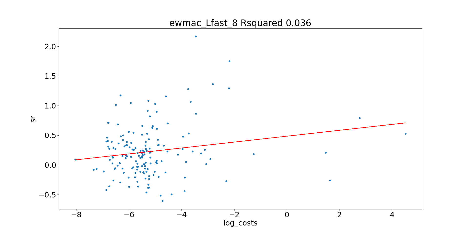
Now to consider the relationship between the cost of an instrument, and the performance of a given trading rule. Each of these scatter plots has one point per instrument; each point shows the SR cost per trade (log) on the x-axis, and the gross SR performance of a given trading rule on the y-axis. I've also added regression lines, and R squared for those regressions.

If the 'no free lunch' rule of equal post cost SR applied, we'd see a positive slope in these charts, whereas if SR were equal pre-cost we'd see a flat line.


So there is something interesting here. For the very fastest trading rules, there is a weak positive relationship (R squared of 0.075) whereby the more expensive an instrument is, the higher the gross SR. That relationship gets monotonically weaker as we slow down, and completely vanishes for the very slowest momentum rule. This does seem to chime with the 'no free lunch' theory; gross profits on very fast momentum are only available for instruments where that would be too expensive to trade.

Perhaps then there is something in the idea that we can use very fast trading rules on expensive instruments, if we can get round the pesky trading costs!


Net SR performance by trading rule versus costs


What happens if we repeat these plots, but with net performance? If the no free lunch (equal post-cost SR) rule is exactly correct, then this should be a horizontal line with no relationship between net SR and the cost of trading a given instruments. Of course if the other hypothesis (equal pre-cost SR) is true, then we'd see a downward sloping line- and because we have log(costs) on the x-axis it would slope downward exponentially. Let's have a look at the very fastest rule:


I haven't dropped a regression line on here, because there clearly isn't a linear relationship. The red vertical line shows the point at which I'd currently stop trading this rule for a given instrument. Everything to the right of this line is an instrument that is too expensive for this trading rule; a SR cost above 0.0031 units. To the right of this line it's clear that we lose more and more money for more expensive instruments; the small improvement in gross SR we saw before for costlier instruments is completely dominated by much higher costs. 

Technically I should allow for the effect of rolls on turnover but in for simplicity I ignore those when drawing the red line, since roll frequency is different for each instrument. They will only have an effect for very expensive instruments at very slow speeds.

But to the left of it things aren't as obvious:


There aren't that many data points here, but there doesn't seem to be much of an upward or downward slope here, which is what we'd expect from the no free lunch theory; to put it another way if costs aren't too high then we can treat the post cost SR as equal, which is a vindication of my forecast weight allocation process. We can confirm that by adding a regression line, but fitting only on the points to the left of the line:


There is a very slight downward slope; indicating that this very fast momentum might be a little closer to the 'equal pre-cost' than 'equal post-cost' hypothesis. But the R squared is very small, and there aren't many data points, reflecting the very small number of instruments that can trade this rule.

Let's continue using  this approach for slower rules:


By the time we get to the very slowest trading rule, it looks much more like the assumption of equal post cost SR is true. The R squared is barely in double figures, so this isn't a very clear result, but it does look like you would want to downweight expensive instruments, as well as removing those that exceed the cost threshold and are to the right of the red line. This remains true even if we're only trading the very slowest EWMAC64 speed on those instruments, which we would be. 

Indeed, if we trust the regression line it looks the cost ceiling for EWMAC64 (and therefore the global cost ceiling to decide whether to trade an instrument at all, in the absence of any cheaper trading rules) should be something like a log cost of -5, or 0.007 SR cost units (the point at which the regression line crosses the x-axis of zero expected SR). 

That's actually a little more conservative than my current global maximum for instrument costs, which is 0.01 SR units (discussed here), but on the other hand the use of dynamic cost penalties means I can probably relax a little on this front.


Optimal trading speed

Let's return to the second set of statements we want to test:

  1. We have a prior belief that the expected pre-cost performance across trading rules for a given instrument is constant. 
  2. Expected post-cost performance across trading rules for a given instrument will be identical.
To put it another way, in a pre-cost world the optimal trading speed will be eithier:
  1. Identical regardless of instrument costs
  2. Faster for more expensive instruments
And in a post-cost world, optimal trading speed will be:
  1. Slower for more expensive instruments
  2. Identical regardless of instrument costs
How do we measure optimal trading speed? This is a bit tricker than just measuring the SR of the rule, since it's effectively the result of a portfolio optimisation. A full blown optimisation would seem a bit much, but just using the EWMAC with the highest SR would be far too noisy. 

I decided to use the following method, which effectively allocates in proportion to SR (where positive):

speed_as_list = np.array([1,2,3,4,5,6])
def optimal_trading_rule_for_instrument(instrument_code, curve_type="gross"):
sr_by_rule = pd.Series([
sr_for_rule_type_instrument(rule_name, instrument_code, curve_type=curve_type)
for rule_name in list_of_rules])

sr_by_rule[sr_by_rule<0] = 0
if sr_by_rule.sum()==0:
return 7.0

sr_by_rule_as_weight = sr_by_rule / sr_by_rule.sum()
weight_by_speed = sr_by_rule_as_weight * speed_as_list
optimal_speed = weight_by_speed.sum()

return optimal_speed

This returns a 'speed number'. The optimal speed number will be 1 (if EWMAC 2 is the best), 2 (if it's EWMAC 4, or something like a combination of EWMAC2,4, and 8 which works out as an average of 4), 3 (EWMAC8), 4 (EWMAC16).... 6 (EWMAC64) or 7 if there are no trading rules with a positive Sharpe (which could be due to very high costs; or just bad luck).


Optimal trading speed with gross SR

Let's repeat the exercise of scatter plotting. Log(costs) of instrument is still on the x-axis, but on the y-axis we have the optimal trading speed, as a number between 1 (fast!) and 6 (very slow!), or 7 (don't bother).

Well this looks pretty flat. The optimal trading speed is roughly 3.5 (somewhere between EWMAC8 and EWMAC16) for very cheap instruments, and perhaps 3 for very expensive ones. But it's noisy as anything. It's probably safe to assume that there is no clear relationship between optimal speed and instrument costs, if we only use gross returns.


Optimal trading speed with net SR

Now let's do the same thing, but this time we find the optimal speed using net rather than gross returns.

As before I've added a red vertical line. Instruments to the right of this are too expensive to trade, even with 100% weight on my slowest trading rule, since their costs would exceed my speed limit of 0.13 SR units per year. 

There are a lot more '7' here, as you'd expect, especially for high cost instruments (which all have negative SR after costs for all momentum), but there are also quite a few lower cost instruments with the same problem. This is just luck - we know that SR by trading rule is noisy, so by bad luck we'd have a few instruments which have negative SR for all our trading rules. 

As we did before, let's ignore the instruments above the red line, and run a regression on what's left over:


That's certainly a strong result, and very much in favour of trading more slowly as instrument costs rise.

However it might be unduly influenced by the '7' points, so let's drop those and see what it looks like without them:
There is still something there, but it's a bit weaker. Roughly speaking, for the very cheapest instruments the optimal trading speed is around 3.5 (something like an equal weight of EWMAC8 and EWMAC16), and for the costliest it's around 5 (EWMAC32, or equivalently an equal weight of 16,32 and 64). 

It's probably worth contrasting this with the weights I currently allocate. Rule turnovers are roughly 42 (EWMAC2), 20, 9, 3.8, 2.3, and 2.1 (EWMAC64). To trade all six rules I would need an instrument SR cost of less than 0.00283 (assuming quarterly rolls), around -5.9 in log space. Such an instrument would have equal weights across all six rules, and therefore a speed number of around 3.5. That is a little faster than the above regression would suggest (-5.9 is closer to an optimal speed number of 4.1), but the regression is very noisy. 

To trade EWMAC64 and nothing else, I'd require an instrument SR cost of less than 0.021 (again assuming quarterly rolls; it would be higher for monthly rolls), or -3.8 in log space. With costs higher than that I couldn't trade anything at all. 

Note that is to the left of the red line, since the red line ignores the effect of rolling on turnover. 

Just EWMAC64 is a speed number of 6, and the regression suggests a speed number of 5.9 with -3.8 log costs. That is a pretty good match.


Summary and implications


Let's deal with the issue of optimal speed first, since the implications here are more straightforward. Broadly speaking it is correct that pre-cost optimal speed is flat, and therefore we should slow down as instruments get more expensive to trade. Although the results are noisy, they suggest that with my current simplistic method for allocating forecast weights I'm spot on with the most expensive instruments, but I might be trading the very cheapest instruments a tiny bit too quickly. However the difference isn't enough to worry about.

Turning to the issue of performance of momentum according to instrument cost, I draw two main conclusions. 

Firstly, the post-cost results suggest that trading rule performance gets worse for more expensive instruments, even if we're trading them slowly. Hence, if I was trading a static system without dynamic optimisation, then I would give consideration to penalising the instrument weight of instruments with high costs (but which were still cheap enough to trade). It's important to note that this is at odds with the approach I've taken before, and discussed in my first book, where I generally set instrument weights without considering costs (assuming post cost SR is equal). Also, my 'cheap enough to trade' bar of 0.01 SR units may be set a little aggressively; 0.007 could be closer to the mark.

However, as I'm currently using dynamic optimisation with a cost penalty, I'm less worried about these issues. This will naturally allocate less to more expensive instruments, and trade them less.

Secondly, the pre-cost performance of momentum versus instrument costs suggests that there is some truth in the idea that more expensive instruments can be traded with fast momentum if you don't have to worry about costs. This is quite a weak result, but I will bear it in mind when I think about 'smuggling in' faster trading rules.

In conclusion, I'm happy that my current pragmatic and simplistic approach to fitting is good enough, but it's been a useful exercise to properly interrogate my assumptions on trading costs and find some surprising results.