Is predicting vol better worth the effort and does the VIX help?

 I'm a vol scaler.

There I've said it. Yes I adjust my position size inversely to vol. And so should you. 

But to this well we need to be able to predict future vol; where the 'future' here is roughly how long we expect to hold our positions for. 

Some people spend a lot of effort on this. They use implied vol from options, high(er) frequency data, GARCH or stochastic vol models. Other people don't spend a lot of effort on this. They look at the vol from the last month or so, and use that. I'm somewhere in the middle (though biased massively towards simplicity); I use an exponentially weighted moving average of recent vol combined with a much slower average.

An obvious question with any research effort is this: is the extra effort worth it? If we were trading options, then sure it would be. But we're not.

In this post I answer that 'is it worth spending time on this nonsense' question and look at the actual improvements we can gain from moving from the most rudimentary vol forecasting to the slightly more complex stuff I do. I also see if we can use a simple indicator of future volatility - the VIX - to improve things further. This was suggested by someone on Twitter(X). 

Is it worth predicting vol better?

I've mentioned this experiement a few times in the past, but I don't think I have ever blogged about it. Basically you run two backtests, one with your normal historic vol estimation, and the other with perfect foresight: basically equal to the ex-post vol over the next 30 days. This will be equal to the theoretical best possible job we could do if we really worked hard at forecasting vol. We can't do any better than a crystal ball. 

Then you check out the improvement. If vol is worth forecasting, there will be a big improvement in performance.

[This is a 'workhorse' test simulation with 100 liquid futures and 4 signals: 40% carry, and 20% in eahc of ewmac 16,32 and 64]

We begin with the simplest possible predictor of vol, a backward looking standard deviation estimate with an infinite window. Essentially this is a fixed vol estimate without any in sample estimation issues. We then compare that to the perfect foresight model.

Let's begin by looking and seeing what the vol outcome is like, this is one month rolling vol estimate (the realised vol of the strategy returns); clearly foresight does a better job of vol targeting.

Above are the cumulated returns. That sure looks like a decent improvement and as the vol of perfect foresight is lower it's better than it looks. It's a half unit improvement in SR points, from 0.76 to 1.24. The skew has dropped off from over 1.0 monthly to 0.12, but you know from my previous posts that small dip in skew won't be enough to destroy the huge CAGR advantage given by this sort of SR premium. The sortino is much better, more than double. 

So the short answer is yes, it's worth predicting vol better. Let's see how 

What size window

The obvious thing to do is to shorten our estimation window from forever to something a little shorter. Here is a graph I like to show people:

The x-axis shows the window size for a historic vol estimator in business days. The y-axis shows the R squared regressing the realised vol for a given future time period against the estimator / predictor of future vol. We're looking for the point on the x-axis that maximises R squared. Each line is a different length of future time period. So for example, to get the best prediction of vol one month ahead (about 21 business days) we look at the purple line for 21 days, and we can see this peaks at around 25 days. 

This is also the highest R squared. We are best at predicting one month vol ahead than other periods, and to do so we should use the previous one month vol (actually slightly more than a month). 

We don't do quite as well predicting shorter periods, and it looks like we might need slightly less data to predict eg 5 day vol. We do worse predicting longer periods, and it looks like we need more data. For 365 days ahead vol, the best R squared is obtained at somewhere between 40 days (around 2 months) and 100 days (around 5 months). 

Note: these are good R squared! In my last post a monthly holding period with an R squared of 0.1 would give us a SR of over 1, which is good. Here we are seeing R squared of over 0.30, which equates to a SR of nearly 2. That is very good - if we were as good at predicting returns as vol our SR would be two!

With that in mind, let's go from an infinite lookback to a 25 day business day lookback and see what happens.

First the rolling vol:

We can already see a fair improvement from the spikiness of the benchmark. How about the returns?

It looks like we are doing better than the benchmark and are competitive with foresight. However some of this is higher vol; our SR is 1.03 which still falls short of the 1.24 of the perfect foresight model, though obviously much better than the benchmark of infinite vol.

To recap:

Infinite previous vol                  SR 0.76

One month simple rolling vol           SR 1.03

Perfect foresight                      SR 1.24

From simple to exponential moving average

Now let's be a little fancier and go to EWM of vol rather than a simple equally weighted measure. This might not get us a better forecast of vol, but we should be smoother. A 36 day span in the pandas EWM function has the same half life as a 25 day SMA.

As before, here's the vol targeting, which is now almost identical:

And for profits....

Again we aren't quite vol matched, but EWM does in fact add a small increment in SR of 0.04 units. Around a quarter of that modest bump comes from lower costs (a saving of around 24 bp a year). 

Infinite previous vol                  SR 0.76

One month simple rolling vol           SR 1.03

One month EWM rolling vol              SR 1.06

Perfect foresight                      SR 1.24

I already looked at this in my book AFTS, but if we combine the standard 25 EWM vol with a very long run average (10 years) of the same vol we get another small bump. This is the vol measure I use myself.

Introducing the VIX

We are still some way short of getting close to perfect foresight vol. So let's do something else, for fun. We know that implied vol should be a good predictor of future vol; accounting for the well known vol premium (we get paid for being short gamma, hence implied is persistently higher than expected future vol).

Here's the simple rolling 25 day standard deviation measure for the S&P 500, and the VIX:

Note: I would like to thank Paul Calluzzo for pointing out a stupid mistake I had made in the first version of this post

A couple of things to notice. Firstly the vol premium is larger after 2008 due to a general level of scaredy-cat-ness, and it sems to have narrowed somewhat inthe last few years. Over the last few years there have been a lot of dumb retail people selling vol and pushing the price down! 

Secondly it looks like VIX tracks rather than predicts increases in risk, at least for those unexpected events which cause the biggest spikes. Which suggests it's predictive power will be somewhat limited.

If we regress future vol on historic vol plus the VIX, the VIX coefficient is 0.14 and the historic vol comes in at 0.71. That suggests historic vol does most of the explaining with VIX not adding much to the party. I get similar results if I put the vol premium (VIX - historic vol) plus historic vol into the regression to reduce potential colinearity. 

Summary

There are significant performance benefits to be gained from forecasting vol well even in a directional system that doesn't trade optionality. Over half of those benefits can be captured by just using the right amount of lookback on a simple historical estimate. Further complexity can probably improve vol targeting but is unlikely to lead to significant performance improvements. Finally, the VIX is not especially helpful in predicting future volatility; mostly this is explained pretty well by historic vol.

Can I build a scalping bot? A blogpost with numerous double digit SR

 I did post recently, from which I shall now quote:

Two minute to 30 minute horizon: Mean reversion works, and is most effective at the 4-8 minute horizon from a predictive perspective; although from a Sharpe Ratio angle it's likely the benefits of speeding up to a two minute trade window would overcome the slight loss in predictability. There is no possibility that you would be able to overcome trading costs unless you were passively filled, with all that implies... Automating trading strategies at this latency - as you would inevitably want to do - requires some careful handling (although I guess consistently profitable manual scalpers do exist that aren't just roleplaying instagram content creators, I've never met one). Fast mean reversion is also of course a negatively skewed strategy so you will need deep pockets to cope with sharp drawdowns. Trade mean reversion but proceed with great care.

Am I the only person who read that and thought.... well if anyone can build an automated scalping bot... surely I can? 

Credit: xkcd (who else?)

To be precise something with a horizon of somewhere around the 4-8 minute mark, but we'd happily go a bit slower (though not too much, lest we hit the dreaded region of mean reversion), or even a bit quicker.

In fact I already have the technology to build one (at least in futures). There's a piece of code in my open source trading system called the (order) stack handler. This code exists to manage the execution of my trades, and implements my simple trading algo, which means it can do stuff like this: 

- get streaming prices from interactive brokers

- place, modify and cancel orders, and check their status with IB

- get fills and write them to a database so I can keep track of performance

- work out my current position and check it is synched with IB

I'll need to do a little extra coding and configuration. For example, I will probably inherit from this class to create my little scalping bot. I will also want to partition my trading universe into the scalped instruments, and the rest of my portfolio (it would be too risky to do both on a given market; and my dynamic optimisation means removing a few instruments from my main system won't cause too much of a headache).

All that leaves then is the "easy" job of creating the actual algo that this bot will run... and doing so profitably.

Some messy python (no psystemtrade required), here, and an sketchy implementation in psystemtrade here.

Some initial thoughts

I'm going to begin with a bit of a brain dump:

So the basic idea is that we start the day flat, and from the current price we set symmetric up and down bracket limit orders. To simplify things, we'll assume those orders are for a fixed number of contracts (to be determined); most likely one but could be more. Also to be determined are the width of those limit orders.

Unlike the (now discredited) slower mean reversion strategy in my fourth book, we won't use any kind of slow trend overlay here. We're going to be trading so darn quick that the underlying trend will be completely irrelevant. That means we're going to need some kind of stop loss. 

If I describe my scalper as a state machine then, it will have a number of states. Let's first assume we make money on a buy.

A: Start: no positions or orders

- Place initial bracket order

B: Ready: buy limit and sell limit

- Buy limit order taken out

C: Long and unprotected: (existing) sell limit order at a profit

- Place sell stop loss below current level

D: Long and protected: (existing) sell limit order at a profit (higher) and sell stop loss order (lower)

- Hit sell limit profit order

E: Flat and unbalanced: sell stop loss order

- Cancel sell stop loss order

A: No positions or orders

Or if you prefer a nice picture:

Lines are orders, black is price, then green because we are long, then black again when we are flat. Red lines are sell order, dotted line is stop loss, green line is buy order.

What happens next: is we reset, and place bracket orders around the current price which is assumed to be the current equilibrium price. Note: if we didn't assume it was the current equilibrium we would have the opportunity to leave our stop loss orders in place. But that also assumes we're going to use explicit stops, which is a design decision to leave for now.

The other profitable path we can take is:

B: Ready: buy limit and sell limit

- Sell limit order taken out

F: Short and unprotected: (existing) buy limit order at a profit

- Place buy stop loss above current level

G: Short and protected: (existing) buy limit order at a profit (lower) and buy stop loss order (higher)

- Hit buy limit profit order

H: Flat and unbalanced: buy stop loss order

- Cancel buy stop loss order

A: No positions or orders

Now what if things go wrong?

D: Long and protected: (existing) sell limit order at a profit (higher) and sell stop loss order (lower)

- Hit sell limit stop loss

J: Flat and unbalanced: sell limit order

- Cancel sell limit order

A: No positions or orders

Alternatively:

G: Short and protected: (existing) buy limit order at a profit (lower) and buy stop loss order (higher)

- Hit buy stop loss limit

K: Flat and unbalanced: buy limit order

- Cancel buy limit order

A: No positions or orders

That's a neat ten states to consider. Of course with faster trading there is the opportunity for async events which will effectively result in some other states occuring, but we'll return to that later. Finally, we're probably going to want to have a 'soft close' time before the end of the day beyond which we wouldn't reopen new positions, and then a 'hard close' time when we would close our existing position irrespective of p&l.

It's clear that the profitability, risk, and the average holding period of this bad boy are going to depend on what proportion of our trades are profitable, and hence on some parameters we need to set:

- position size

- initial bracket width

- distance to stop loss

... some numbers we need to know:

- contract multiplier and FX

- commissions and exchange fees

- the cost of cancelling orders 

... and also on on some values we need to estimate:

- volatility (we'd probably need a short warm up period to establish what that is)

- likely autocorrelation in prices

Note: We're also going to have to consider tick size, which we need to round our limit orders, but also in the limit will result in a minimum bracket width of two ticks (assuming that would still be a profitable thing to do).

Further possible refinements to the system could be to avoid trading if volatility is very high, or is in a period of adjustment to a higher level (which depending on time scale can basically mean the same thing). We could also throw in a daily stop loss on the scalper, if it loses more than X we stop for the day as we're just 'not feeling it'.

Another implementation detail that springs to mind is how we handle futures rolls; since we hope to end the day flat this should be quite easy; we just need to make sure any rolls are done overnight and not trade if the system is in any kind of roll state (see 'tactics' chapter in AFTS and doc here).

Living in a world of OHLC

Now as you know I'm not a big fan of using OHLC bars in my trading strategies -  I normally just use close prices. I associate using OHLC prices and creating candle stick charts with the sort of people who think Fibbonaci is a useful trading strategy, rather than the in house restaurant at a london accountants office. 

However OHLC do have something useful to gift us, which is the concept of the likely trading range over a given time period (the top and the bottom of a candle). 

Let's call that range R, and it's simply the difference between the highest and lowest prices over some time horizon H (to be determined). We can look at the most recent time bucket, or take an average over multiple periods (a stable R could be a good indication of stable volatility which is a good thing for this strategy). So for example if we're looking at '5 minute bars' (I'll be honest it takes an effort to use this kind of language and not throw up), then we could look at the height of the last bar, or take a (weighted?) average over the last N bars.

Now to set our initial bracket limit orders. We're going to set them at (R/2)*F above and below the current price. Note that if F=1, we'll set a bracket range which is equal to R. Given we're assuming that R is constant and represents the expected trading range, we're probably not going to want to set F>=1.  Smaller values of F mean we are capturing less of the spread, but we're exposed for less time. Note that setting a smaller F is equivalent to trading the same F on a smaller R, which would be a shorter horizon. So reducing F just does the same thing as reducing R. For simplicity then, we can set F to be some fixed value. I'm going to use F=0.75.

Finally, what about our stop losses? It probably makes sense to also scale them against R. Note that if we are putting on a stop loss we must already have a position on, which means the price has already moved by (R/2)*F. The remaining price "left" in the range is going to be (R/2)*(1-F); to put it another way versus the original 'starting' price we could set our stop loss at (R/2) on the appropriate side if we wanted to stop out at the extremes of the range. But maybe we want to allow ourselves some wriggle room, or set a stop closer to our original entry point. Let's set our stop at (R/2)*K from the original price, where K>F. 

Note this means our (theoretical!!!) max loss on any trade is going to be (R/2)*(K-F). For example, if F=0.75 and K=1.25 (so we place our stops at the extreme of the range), then the most we can lose if we hit our stop precisely is R/4.

Back of the envelople p&l

We're now in a position to work out precisely what our p&l will be on winning trades, and roughly (because stop loss) on losing trades. Let's ignore currency effects and set the multiplier of the future to be M (the $ or otherwise value of a 1 point price move). Let's set commission to C and also assume that it costs C to cancel a trade (the guidance on trade cancelling cost in interactive brokers docs is vague, so best to be conservative). In fact it makes more sense to express C as a proportion of M, c.

Finally we assume we're going to use an explicit stop loss order rather than implicit which means paying a cancellation charge.

win, W = R*F*M - 3C = R*F*M - 3Mc = M(R*F - 3c)

loss, L = -(K-F)*M*R/2 - 3C = -M[(K-F)*R/2 + 3c)

I always prefer concrete examples. For the SPY micro, M=$5, C=$0.25, c=0.05 and let's assume for now that R=10. I'll also assume we stick to F=0.75 and K = 1.25. So our expected win is:

W = $5 * (10*0.75 - 3*0.05) = $36.75

L = -5*[(1.25 - 0.75)*10/2 +3*0.05] = -$13.25

Note that in the absence of transaction costs the ratio of W to L would be equal to 2F / (F-K) which in this case is equal to 3. Note also that the breakeven probability of a win for this to be a profitable system is L / (L-W) which would be 0.25 without costs, but actually comes out at around 0.265 with costs.

We can see that setting K will change the character of our trading system. The system above is likely to be quite positive skew (breakeven probability). If we were to make K smaller, then we'd have more wins but they are likely to be smaller, and we'd get closer to negative skew.

Introducing the speed limit

Readers of my books will know that I am keen on something called the 'speed limit'; the idea that we shouldn't pay too much of our expected return on costs. I recommend an absolute maximum of 1/3 of returns paid out on costs; in practice eg for my normal trading strategy I pay about 1% a year and hope to earn at least ten times on that.

On the same logic, I'm not sure I'd be especially happy with a strategy where I have to pay up half my profits in costs even on a winning trade. Let's suppose the fraction of gross profit I am happy to pay is L, then:

3Mc / R*F*M = L

R = 3c / LF

For example, if L was 0.1 (we only want to pay 10% of our costs), then the minimum R for F=0.75 on the S&P 500 with c=0.05 would be 3*.05 / (0.1 * 0.75) = 2

In practice this will put a floor on the horizon chosen to estimate R; if H is too short then R won't be big enough. The more volatile the market is, the shorter the horizon will be when R is sufficiently large. However we would want to be wary of a longer horizon, since that would push us towards a holding period where autocorrelation is likely to turn against us (getting up towards 30 minutes).

But as we will see later, this crude method significantly understimates the impact of costs as it ignores the cost of losing trades. In practice we can't really use the speed limit idea here.

Random thought: Setting H or setting R?

We can imagine two ways of running this system:

- We set R to be some fixed value. The trading horizon would then be implicit depending on the volatility of the market. Higher vol, shorter horizon. We might want to set some limits on the horizon (this implies we'll need some sensitivity analysis on the relationship between horizon and the ratio of R and vol). For example, if we go below a two minute horizon we're probably pushing the latency possibilities of the python/ib_insyc/IB execution stack, as well as going beyond the horizon analysed in the arvix paper. If we go above a fifteen minute horizon, we're probably going to lose mean reversion again as in the arvix paper. 

- We set the horizon H at some fixed value, and estimate R. We might want to set some limits on R - for example the speed limit mentioned above would put a lower limit on R. 

In practice we can mix these approaches; for example estimating R at a given horizon at the start of each day (perhaps using yesterdays data, or a warm up period), and then keeping it fixed throughout the day; or maybe re-estimating once or twice intraday. We can also at this point perhaps do some optimisation on the best possible value of H; the period when we see the best autocorrelation.

Simulation

Right, shall we simulate this bad boy? Notice I don't say backtest. I don't have the data to backtest this. I'm going to assume, initially, very benign normal distribution returns that - less benign - has no autocorrelation.

Initially I'm going to use iid returns, which is conservative (because no autocorrelation) but also aggresive (no jumps or gaps in prices, or changes in volatility during the day). I'm also going to use zero costs and cancellation fees, and optimistically assume stop losses are filled at their given level. We're just going to try and get a feel for how changing the horizon, and K affect return distribution. I'm going to re-estimate R throughout the day with a fixed horizon, but given the underlying distribution is random this won't make a huge amount of difference.

The distribution is set up to look a bit like the S&P 500 micro future; I assume 20% annualised daily vol and then scale that down to an 8 hour day (so no overnight vol). That equates to 71.25 units of price of daily vol, assuming the current index level of ~5700. I will simulate one day of ten second price ticks, do this a bunch of times, and then see what happens. The other parameters are those for the S&P micro: contract multiplier $5, tick size $0.25, and I also use a single contract when trading.

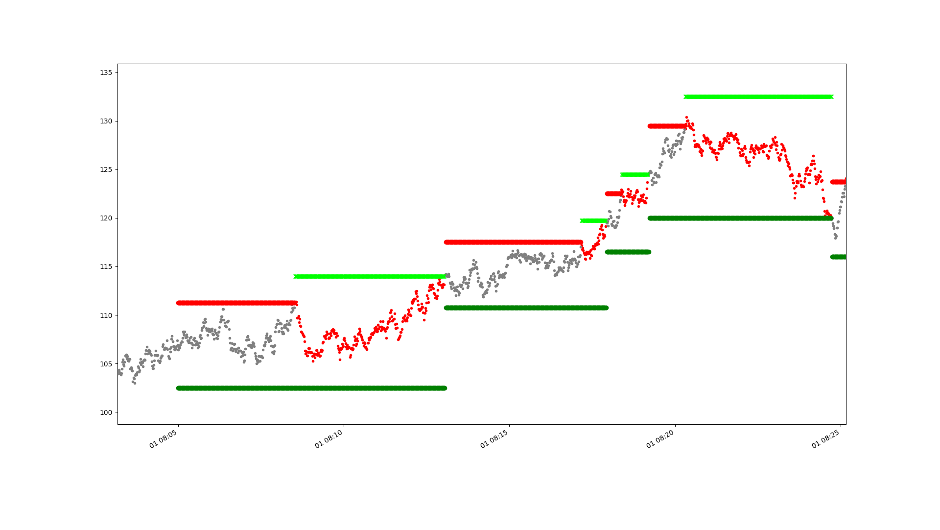
The simulations can be used to produce pretty plots like this which show what is going on quite nicely:

The price is in grey, or red when we are short, or green if long. The horizontal dark red and green lines are the initial take profit bracket orders. You can see we hit one early on and go short. The light green line is a buy stop loss (there are no sell stop losses in this plot as we're only ever short). You can see we hit that, so our initial trade fails. We then get two short lived losing trades, followed by a profitable trade near the end of the period when the price retraces from the red bracket entry down to the green take profit line.

Here's a distribution of 5000 days of simulation with a 5 minute horizon, and K=1.25 (with F=0.75):

Well it loses money, which isn't great. The loss is 0.4 Units of the daily risk on one contract (daily vol 71.25 multiplied by multiplier $5). And that's with zero costs and optimistic fills remember. Although there is a small point to make, which is that this isn't a true order book simulator. I only simulate a single price to avoid the complexity of modelling order arrival. In reality we'd gain a little bit from having limit orders in place in a situation where the mid price gets near but doesn't touch the limit order. Basically we can 'earn' the bid-ask bounce. 

The distribution of daily returns is almost perfectly symettrical, obviously that wouldn't be true of the trade by trade distribution.

What happens if we set a tighter stop, say K=0.85?

Now we're seeing profits (0.36 daily risk units) AND some nice positive skew on the daily returns (which have a much lower standard deviation of about 0.40 daily risk units). Costs are likely to be higher though, and we'll check that shortly. Note we have a daily SR approaching 1.... which is obviously bonkers- it annualises to nearly 15!!! Incredible bearing in mind there is no autocorrelation in the price series at all here. But of course, no costs.

What happens if we increase the estimate period for R to 600 seconds (10 minutes), again with K=0.85:

Skew improves but returns don't. Of course, costs are likely to fall with a longer horizon.

An analysis of R and horizon

Bearing in mind we know what the vol of this market is (71.25 price units per day), how does the R measured at different horizons compare to that daily vol? Note this isn't affected by the stoploss or costs.

At 60 seconds, average R is 4.6, in daily vol units: 0.065

At 120 seconds, .... R in vol units: 0.10

At 240 seconds, ...  R in vol units: 0.15

At 360 seconds, ...  R in vol units: 0.19

At 480 seconds, ...  R in vol units: 0.22

At 600 seconds, ... R in vol units: 0.25

At 900 seconds, ... R in vol units: 0.31

This doesn't quite grow at sqrt(T) eg T^0.5, but at something like T^0.59.

Footnote: even the smallest value of R here is greater than the minimum calculated earlier based on our speed limit. Of course that wouldn't be true for every market. 

Now with costs

Now let's include costs in our analysis. I'm going to assume we pay $0.25 per contract, and the same to cancel, which is c=0.05 as a proportion of the $5 multiplier. In the following tables, the rows are values of H, and the columns are values of K. For each I run 5000 daily simulations and take the statistics of the distribution of daily returns.

First the average daily returns, normalised as a multiple of the daily $ risk on one contract (71.25 * M = $356.25 ). Note I haven't populated the entire table, as there is no point focusing on points which won't make any money (with the exception of those we've already looked at).

H / K    0.8     0.85    0.92       1.0    1.25   

120      0.62    0.26   -0.16     -0.53   -1.08

240      0.37    0.09   -0.21     -0.44   -0.70  

300      0.30    0.04   -0.22             -0.60

600      0.14   -0.04

900      0.07   -0.05                     -0.25                     

Note we've already seen some of these values before pre-cost; H=300, K=1.25 was -0.4 (now -0.60), H=300, K=0.85 was 0.36 (now 0.044), and H=600, K=0.85 was 0.13 (now -0.04). So we lose about 0.2, 0.32 and 0.17 in daily risk units in costs. We lose more in costs if H is smaller (as we trade more often) and with a tighter stoploss (as we have more losing trades, and thus trade more often). To put it another way, we lose 1 - (0.044/0.36) = 78% of our gross returns to costs with H=300, K=0.85 (which is a darn sight more than the speed limit would like!).

Note: even with a 5000 point bootstrap there is some variability in these numbers; for example I ran the H=120/K=0.8 twice and on the other occasion got a mean of over 0.8.

Standard deviations, normalised as a multiple of the daily $ risk on one contract:

H / K    0.8     0.85    0.92    1.0     1.25   

120      0.34    0.37    0.41    0.46    0.58

240      0.35    0.39    0.45    0.50    0.63

300      0.35    0.40    0.47            0.65

600      0.35    0.41

900      0.35    0.41                    0.67

These are mostly driven by the stop; with longer lookbacks increasing it slightly but not by much.

Annualised daily SR:

H / K    0.8     0.85    0.92     1.0   1.25   

120      28.8   11.4    -6.0    -17.7  -29.7

240      17.0    3.8    -7.7    -14.1  -17.7

300      13.9    1.77   -7.5           -14.6

600      6.3    -1.53

900      3.24   -1.98                   -5.9

These numbers are... large. Both positive and negative.

Skew:

H / K    0.8     0.85    0.92   1.0   1.25 

120      0.16    0.12    0.09   0.07  0.03

240      0.18    0.22    0.15   0.13  0.03

300      0.30    0.16    0.19         0.10

600      0.42    0.27

900      0.54    0.35                 0.08

As we'd expect, tighter stop is better skew. But we also get positive skew from longer holding periods.

With more conservative fills

So it's simple, right, we should run a short horizon (say H=120) with a tight stop (say 0.8, which is only 0.05R away from the initial entry price).  It does seem that a tight stop is the key to success; the SR is very sensitive to the stop increasing in size, 

But it's perhaps worth examining what happens to the SR of such a system as we change our assumptions about costs and fills. With very tight stops, and short horizons, we are going to get lots more trades (so costs have a big impact), and hit many more stops; so the level at which we assume they are filled is critical. Remember above I've assumed that stops are hit at the exact level they are set at.

Z: Zero costs, stop loss filled at limit, take profit filled at limit 

CL: Costs, stop loss filled at limit, take profit filled at limit

CP: Costs, stop loss filled at next price, take profit filled at limit

CLS: Costs, stop loss filled at limit + slippage, take profit filled at limit

CPS: Costs, stop loss filled at next price + slippage, take profit filled at limit

CLS2: Costs, stop loss filled at limit + slippage, take profit filled at limit - slippage

CPS2: Costs, stop loss filled at next price + slippage, take profit filled at limit - slippage 

Two sided slippage (CSL2, CPS2)- means we assume we earn 1/2 a tick on take profit limit orders (assumes a 1 tick spread, which is configurable), and have to pay 1/2 a tick on stop losses (of which there will be many more with such tight stops). Essentially it's the approximation I use normally when backtesting, and tries to get us closer to a real order book. There's also a more pessimistic one sided version of these (CLS, CPS) where we only apply the negative slippage. 

Here are the Sharpe Ratios, different strategies in columns (I've just gone for a selection of apparently profitable), different cost assumptions in rows (numbers are comparable with each other as used same random seed, but not comparable with those above):

H/K: 120/0.8      300/0.8      900/0.8      120/0.85      300/0.85

ZL:    48.6          23.9          7.5           29.6        10.4

CL:    28.9          14.1          3.2           11.9         2.5

CLS2:  32.2          15.4          3.7           16.5         4.1

CLS:    7.0           2.9          -1.7          -7.2         -6.2

CP:    -120           -69          -35           -114         -59

CPS2:  -115           -66          -34           -109         -56

CPS:   -129           -75          -38           -123         -64

Well we know that zero costs (ZL) and costs with stop losses being hit exactly (CL) are probably a pipe dream, so then it's a question of which of the other five options gets closest to the messy reality of a real life order book as far as executing the stop loss orders goes. Clearly using the next price(CP*) is an absolute killer to performance with the biggest damage done as you would expect on the tightest stops and shortest horizons where we lose up to 140 units of annualised SR. We're not going to be able to do much unless we assume we can get near the limit price on stop loss orders (*L*).

If we assume, reasonably conservatively, that we receive our limits on stop profit orders without benefitting from bid-ask bounce, but have to pay slippage on our stop losses - which is CLS - there are still two systems that survive with high positive SR. 

Interactive brokers provides synthetic stop losses on some markets; whether it's better to use these or simulate our own stops by placing aggressive market orders once we are past the stop level is an open question.

Note that even the most optimistic of these (CSL2) sees us losing half or more of the pre-cost returns, again hardly what I usually like to see but I guess I could live with an annualised SR of over 7 :-)

Can't we do better

All of the above assumes prices are a pure random walk.... but the original motivation was the fact that prices in the sort of region I'm looking at appear to be mean reverting. Which would radically improve the results above. It's easy to generate autocorrelated returns at the same frequency as your data, but I'm generating returns every 10 seconds whilst the autocorrelation is happening at a slower frequency. We'd have to use something like a brownian bridge to fill in the other returns, or also assume autocorrelation happens at the 10 second frequency, which we don't know for sure and would flatter us too much. The final problem is that I don't actually have figures to calibrate this with; the arvix paper doesn't measure autocorrelation.

Since I've already spent quite a lot of time digging into this, I decided not to bother. Ultimately a system like this can only really be tested by trading it; as that's also the only way to find out which of the assumptions about fill prices is closest to the truth. Since the SR ought to be quite high, we should be able to work out quite quickly if this is working or not. 

System choice in tick terms

This then brings me back to which is the best option of H and K to trade.

Remember from above that the average R expressed in daily vol units varies between 0.10 (for H=120 seconds) up to 0.31 (H=900 seconds). If we use K=0.8 (with L=0.75) then we'll have a stop of 0.05R, which will be 0.05*0.10 = 0.005 times daily vol. To put that in context, if S&P 500 vol is around 1%, or call it 60 points a day, then R=6 price units, and our stop will be just 0.3 price points away.. which is just over one tick (0.25)! You can now see why the tight K, short horizon, systems were so sensitive to fill assumptions. For the slowest system in the second set of analysis above, H=300/K=.85, as a stop of 0.1R with R~0.17 we get up to four ticks between our take profit and stop loss limits.

We're then faced with the dilemna of hoping we can actually get filled within a tick of that level (and if it doesn't will absolutely bleed money), or slowing down to something that will definitely lose money unless we get mean reversion (but won't lose as much). 

If we were to say we wanted to see at least 10 ticks between take profit and stop loss, then we're looking at something like H=900, K=0.87; or H=120, K=1; or somewhere in between.  The former has a less bad SR, better skew and lower standard deviation - basically a tighter stop on a longer horizon is better than a looser stop on a shorter one.

Next steps

My plan then is to actually trade this, on the S&P with H=900 and K=0.87. I'll come back with a follow up post when I've done this! 

Postscript: It didn't work

I should probably try on less liquid instruments with larger spreads at some point.

The State Of Vol

 I'm sometimes asked where I get my ideas for new trading strategies from. The boring truth is I rarely test new trading strategies, and I mostly steal ideas when I feel in the mood. Today for example I saw this tweet post on twitter X:

Think high market volatility leads to high returns? No. Periods with high market volatility are followed by high volatility, but not necessarily better returns. A volatility effect through time. Check out the graph below, based on the US equity market from 1927 to 2023. The… pic.twitter.com/23rrTwIf9O

— Pim van Vliet (@paradoxinvestor) October 2, 2023

The original paper is here  (requires subscription or academic institution membership)

Now I've written in the past about how volatility levels affect the profits of trading strategies, in particular momentum where there is a pretty striking effect (see my new book Advanced Futures Trading Strategies [AFTS] for more info), and I've also written about how the level of past vol affects future vol (and indeed, this incredible predictability of vol is a cornerstone of the inverse volatility sizing formula that lies at the heart of my trading strategies), but I don't think I've ever written about the level of volatility's effect on future price movements. 

There is quite a simple story here which if you can see the paper is in figure 1: absolute returns are pretty flat across different vol regimes, and because vol is pretty autocorrelated from month to month, we'd expect return/vol to be higher if recent vol was lower. To put it another way, there is a link here with my previous post about CAPM; this story is sort of about the time series version of CAPM in which higher vol should be rewarded with higher returns (and hence Sharpe Ratios should not show any pattern conditional on relatively volatility levels), and the opposite happens in single stocks in an analogy to the fact that CAPM doesn't work in cross section for single stocks, in fact we should 'bet against beta' and buy low beta stocks.

But the paper is written for single stocks; a risky asset, and one with some idiosyncratic distributional features. Will the results hold for the wider universe of futures markets? 

Data and definitions

I am not interested in reproducing the results in the paper since I'm more concerned with whether this is a profitable trading strategy sitting within my usual framework, so I will do things a bit differently.

I use my usual set of futures markets, after removing duplicates (eg micro and mini versions, or cross listings) it comes in at 211 instruments. Data goes back to 1970, and I use my standard vol estimate calculated in % terms, which I divide by an exponential moving average of the same with a 10 year vol halflife to get a relative vol measure. If this is 1, then the vol we're seeing is going to be typical of the level over the last couple of decades or so, if it's higher than 1 then the vol is higher, and so on. Again readers of AFTS will recognise this measure. The paper doesn't quite do this; it just looks at the level of vol versus the in sample historic distribution. This means we can't use that forecast as a trading signal.

For the y-axis of response, I will use the returns in the following month normalised by the volatility estimate (in price differences this time) at the beginning of the month for reasons I have discussed before. As I'm trading futures, this is also the Sharpe Ratio. The original paper uses a straight one month moving window of returns for vol estimation, and the pure ex-post Sharpe Ratio using the realised vol in the following month, so some small difference there. However because of the autocorrelation of vol, it shouldn't affect things too much; if anything my results probably should be a bit better because I'm dividing an unknown future estimate of mean by a known current estimate of standard deviation to get Sharpe Ratio, rather than having unknown mean/unknown sigma.

The original papers uses single stocks, I use a massive variety of futures allowing me to see if this effect persists at the stock index level and for other asset classes. 

Some comparable graphs

Let's start with producing the same kind of graphs as in the paper. So each month I look at the current level of vol versus it's historic average, and then rank it on an in sample basis (yes I know, but for the time being...), and then bucket the ranking into quintiles. I measure the risk adjusted return in the following month and take a median of those Sharpe Ratios; medians being somewhat more robust than mean.

Here is the result for the S&P 500:

I use the same ordering; 1 on the left is the lowest quantile of vol, 5 on the right is the highest. That picture is not quite as compelling as the original paper; but ignoring the 2nd bar it has the right pattern: higher recent vol means lower risk adjusted returns in the following month. Nevertheless we are only using 492 data points compared to the thousands we can get with single stocks; plus I am suspicous of anyone that uses a single instrument to prove anything, so let's expand out to all equity futures (with months stacked, which will give a higher weight to instruments with more history):

That is .... not what we'd hoped for.

The name is Bond:

Not great. What about Vol (VSTOXX, VIX)?

OK only two markets, but there is an apparent reverse effect here. You don't want to be long vol on average, but perhaps the worst time to be is when vol of vol is very low.

FX:

At best noise, at worst the reverse of what we expect.

Metals

That is the strongest, wrong way round, effect we have seen. Agricultural:

Just noise really. And finally energies:

The wrong way round, and inconsistent.

It's probably futile, but what happens if we pool our results across all markets?

There could be a story there- higher vol means higher risk adjusted returns, unless vol is very high; or we could be looking at the aggregated result of jamming together instruments that behave very differently*, plus a bunch of instruments that are just noise. 

[* it looks like markets fall into two camps, one where the effect is the 'right way' round (high vol, lower returns; perhaps the S&P 500 is here), others where it is the wrong way (most strikingly, vol), and the third of the two camps doesn't really have a strong effect]

Just to give a point of comparison, here's the bucket plot if I replace the ratio of vol with the level of the 32/128 day momentum forecast level (something we know is very successful as a forecast at a portfolio level, although it is weak in say equities):

Clearly this vol effect is not as strong as momentum.

A trading rule

Although the results aren't what we expect, this could be profitable as a 'wrong way round' rule, which buys when vol is higher, and sells when vol is lower. This won't work for very high vol (since quintile 5 shows a worse return for quintiles 2,3 and 4, but then we would hit forecast capping up there anyway. That isn't much different to what happens with faster momentum rules anyway; if you plot response versus forecast level it's not as good for extreme forecasts (see AFTS for more).

In my first book, Systematic Trading, I said that implementing a rule as a wrong way rule after discovering it is a form of data mining so bear in mind that the backtest results here will effectively be overstated [in reality, you couldn't have implemented this rule until enough historical evidence that the effect was the 'wrong' way round existed; until that moment of statistically significant realisation we would eithier be trading the money losing 'right way round' rule, or a combination of the two, eithier of which is inferior to being all in on 'wrong way round' from the start of the backtest].

I'd add a couple of tweaks as well; firstly rather than quantile buckets which are too coarse and in sample; I will use the percentile of the ratio versus historic levels as the forecast (the same approach I use for the volatility overlay rule in AFTS) , and also chuck in my standard ewm(span=10) smooth to reduce noise on what should be a monthly holding forecast (this reduces turnover from 25 times a year to 10 times without affecting profitability).

Before continuing, it might be worth thinking about how this interacts with the volatility overlay on a trend following rule (which cuts exposure long or short when vol is high).

• If vol is low, we'd be SHORT from a vol rule
• ... and we'd have a stronger trend following signal
• if markets are trending up we'd be net flat
• If markets are trending down we'd have a strong sell
• If vol sits in the middle, we'd be FLAT from a vol rule
• .... and we've have an unadulterated trend signal
• If markets are trending up we'd be long
• If markets are trending down we'd be short
• If vol is high, we'd be LONG from a vol rule
• .... and have a weaker trend following signal
• If markets are trending up we'd be modestly long
• If markets are trending down we'd be flat

Clearly this will work differently for risk on/risk off markets; risky markets like equities will most probably go up with low vol and down with high vol, thus occupying the two lines shown with italics. In these situations we'd have no position on (assuming these are the only two trading rules we're using). Since trend following doesn't work super well in equity indices, this might improve our lives somewhat.

Risk off markets, the most extreme of which is VIX/VSTOXX, will occupy the lines in bold as they have high vol when they are going up, and low vol vol the way down. Notice that this will introduce a short bias (modest long on the way up, strong short on the way down); since these markets tend to lose money on the long side again we might expect a benefit here.

Other markets - which form the majority of futures instruments - will be less clear, so let's see how it goes.

Here's the code for the purely backward looking vol quantile calculation, and the actual trading rule:

def get_vol_quantile_points(self, instrument_code):
    self.log.debug("Calculating vol quantile for %s" % instrument_code)
    daily_vol = self.parent.rawdata.get_daily_percentage_volatility(instrument_code)
    ten_year_vol = daily_vol.rolling(2500, min_periods=10).mean()
    normalised_vol = daily_vol / ten_year_vol

    normalised_vol_q = quantile_of_points_in_data_series(normalised_vol)

    return normalised_vol_q

def quantile_of_points_in_data_series(data_series: pd.Series) -> pd.Series:
    ## With thanks to https://github.com/PurpleHazeIan for this implementation
    numpy_series = np.array(data_series)
    results = []

    for irow in range(len(data_series)):
        current_value = numpy_series[irow]
        count_less_than = (numpy_series < current_value)[:irow].sum()
        results.append(count_less_than / (irow + 1))

    results_series = pd.Series(results, index=data_series.index)
    return results_series

def vol_rule(vol_quantile_points: pd.Series, smooth: int = 10):
    # vol quantile points sits in space 0 to 1.0
    raw_forecast = (vol_quantile_points - 0.5) * 40  ## sits in space -20 to +20
    smoothed_forecast = raw_forecast.ewm(span=smooth).mean()
    return smoothed_forecast

System test

I'm testing this using my current trading system with 147 instruments and relevant instrument weights. I'll be using the 'static' rather than 'dynamically optimised' flavour of the system, to get a feel for pure performance before the noise added by optimisation. This also means I'm going to put in an unrealistically large slug of capital, and remove a few markets that are too expensive to trade, bringing me down to 138 markets. I estimate instrument weights and the IDM (which peaks at 2.15) using my usual optimisation defaults.

To begin with, let's look at the performance of the vol strategy by itself. You're all dying to see it, so here is the money shot with the full account curve before and after costs:

Well it's not terrible but it's not amazing eithier. The Sharpe is a mere 0.10, which is not exactly knocking it out of the park... at best we've tapped the ball and it's dribbled a few feet away. 

Can this thing add value when combined with momentum (particularly given the discussion above)? Let's keep it simple and just use a single ewmac rule, 16/64. Correlation between the rules is actually a little negative, so let's do some god-awful in sample fitting and allocate 10% of our portfolio to the new vol rule.

It's not really worth plotting as these two systems will both look pretty similar, but this relatively small allocation to our new putative signal does indeed push up the Sharpe Ratio from 1.10 to 1.15, with the Sortino rising by a similar amount. Costs are slightly reduced, skew falls slightly (from 0.55 to 0.48), but the more robust lower tail ratio is unchanged (see AFTS for a definition). 

Summary

It does seem like the predictive effect of vol in single equities isn't replicated across the futures universe; if anything the effect is reversed although it is not as strong as in the original paper. Rather than buying instruments with lower vol to get higher risk adjusted returns, we should do the opposite. Rather than 'time series CAPM' failing, and a 'bet against time series standard deviation levels', we in fact see an even stronger 'time series CAPM' where risk adjusted returns aren't constant with relative vol levels, but actually improve when volatility is relatively high.

If we use this idea to construct a simple trading rule the result is not the world's greatest standalone signal. But there does seem to be some promise in adding it to a trend following strategy due to it's negative correlation.

Percentage or price differences when estimating standard deviation - that is the question

In a lot of my work, including my new book, I use two different ways of measuring standard deviation. The first method, which most people are familiar with, is to use some series of recent percentage returns. Given a series of prices p_t you might imagine the calculation would be something like this:

Sigma_% = f([p_t - p_t-1]/p_t-1, [p_t-1 - p_t-2]/pt-2, ....)

NOTE: I am not concerned with the form that function f takes in this post, but for the sake of argument let's see it's a simple moving average standard deviation. So we would take the last N of these terms, subtract the rolling mean from them, square them, take the average, and then take the square root.

For futures trading we have two options for p_t: the 'current' price of the contract, and the back adjusted price. These will only be the same in the days since the last roll. In fact, because the back adjusted price can go to zero or become negative, I strongly advocate using the 'current' price as the denominator in the above equation, and the changein back adjusted price as the numerator. If we used the change in current price, we'd see a pop upwards in volatility every time there was a futures roll. So if p*_t is the current price of a contract, then:

Sigma_% = f([p_t - p_t-1]/p*_t-1, [p_t-1 - p_t-2]/p*t-2, ....)

The alternative method, is to use some series of price differences:

Sigma_d = f([p_t - p_t-1], [p_t-1 - p_t-2], ....)

Here these are all 

If I wanted to convert this standard deviation into terms comparable with the % standard deviation, then I would divide this by the current price (*not* the backadjusted price):

Sigma_d% = Sigma_d / p*_t

Now, clearly these are not going to give exactly the same answer, except in the tedious case where there has been no volatility (and perhaps a few, other, odd corner cases). This is illustrated nicely by the following little figure-ette (figure-ine? figure-let? figure-ling?):

import pandas as pd
perc =(px.diff()/pxc.shift(1)).rolling(30, min_periods=3).std()
diff = (px.diff()).rolling(30, min_periods=3).std().ffill()/pxc.ffill()
both = pd.concat([perc,diff], axis=1)
both.columns = ['%', 'diff']

The two series are tracking pretty closely, except in the extreme vol of late 2008, and even they aren't that different. 

Here is another one:

That's WTi crude oil during COVID; and there is quite a big difference there. Incidentally, the difference could have been far worse. I was trading the December 2020 contract at the time... the front contract in this period (May 2020) went below zero for several days.

Now most people are more familiar with % standard deviations, which is why I have used it so much, but what you may not realise is that the price difference standard deviation is far more important.

How come? Well consider the basic position sizing equation that I have used throughout my work:

N = Capital × τ ÷ (Multiplier × Price × FX rate × σ_% )

(This is the version in my latest book, but very similar versions appear in my first and third books). Ignoring most things we get:

N = X ÷ (Price × σ_%)

So the number of contracts held is proportional to one divided by the price multiplied by the percentage standard deviation estimate. The price shown is, if you've been paying attention, the current price not the back adjusted one. But remember:

Sigma_d% = Sigma_d / p*_t

Hence the position is actually proportional to the standard deviation in price difference terms. We can eithier estimate this directly, or as the equation suggests recover it from the standard deviation in percentage terms, which we then multiply by the current futures price.

As the graphs above suggest, in the majority of cases it won't make much difference which of these methods you choose. But for the corner case of prices close to zero, it will be more robust to use price differences. In conclusion: I recommend using price differences to estimate the standard deviation.

Finally, there are also times when it still makes sense to use % returns. For example, when estimating risk it's more natural to do this using percentages (I do this when getting a covariance matrix for my exogenous risk overlay and dynamic optimisation). When percentage standard deviation is required I usually divide my price difference estimate by the absolute value of the current futures price. That will handle prices close to zero and negative prices, but it will result in temporarily very high % standard deviations. This is mostly unavoidable, but at least the problem is confined to a small part of the strategy, and the most likely outcome is that we won't take positions in these markets (probably not a bad thing!).

Footnote: Shout out to the diff(log price) people. How did those negative prices work out for you guys?

Vol targeting: A CA(g)R race

Regular listeners to the podcast I ocasionally co-host will know that I enjoy some light hearted banter with some of my fellow podcasters, many of whom describe themselves as 'pure' trend followers, whilst I am an apostate who deserves to be cast into the outer darkness. My (main) sin? The use of 'vol targeting', an evil methodology not to be found in the original texts of trend following, or even in the apocrypha, and thus making me unworthy. In brief, vol targeting involves adjusting the size of a trade if volatility changes during the period that you are holding it for. A real trend follower would maintain the position in the original size.

(But we agree that the initial position should be sized according to the risk when the trade is entered into)

I've briefly discussed this subject before, but I thought it might be worthwhile to have another look. In particular, the pure trendies generally object to my use of Sharpe Ratios (SR) as a method for evaulating trading performance. And you know what - they are right. It doesn't make much sense to use SR when two or more trading strategies have different return distributions. And it's well known that purer trend following has a more positive skew than the vol targeted alternative, although that effect isn't as large when you look at returns as you might expect. Also, for what it's worth, purer trend following has fatter tails, both left and right.

The reason I use Sharpe Ratio of course is that it's a risk adjusted return, which makes in invariant to the amount of leverage. So if we're not going to use risk adjusted returns, then what? I'm going to do the following, and pick the strategy with the best annualised compounding return at the optimal leverage level for that strategy. Because positively skewed strategies can have higher leverage than those with less skew (see my first book Systematic Trading for some evidence), this will flatter the purer form of trend following.

** EDIT 29th June - added 3 slower strategies and turnover statistics **

The systems

What I'm trying to do here is to isolate the effect of vol targeting by making the trading systems as close as possible to each other. 

Each of the alternatives will use a single kind of moving average crossover trading rule(s), but the way they are used will be rather different:

1. 1E1S'One entry, one stop' (binary, no vol targeting). We enter a trade with a full sized fixed position when the crossover goes long or short, and we exit when we hit a trailing stop loss. We reenter the trade when the crossover has changed signs. The size of the stop loss is calibrated to match the turnover of the entry rule (see here and here). The stop loss gap remains fixed throughout the life of the trade, as does the position size. This is basically the starter system in chapter six of Leveraged Trading.
2. 1E1E 'One entry, one exit' (binary, no vol targeting). We enter a trade with a full sized fixed position when the crossover goes long or short, and we exit when the crossover has changed signs, immediately opening a new position in the opposite direction. The position size remains unchanged. This is the system in chapter nine of Leveraged Trading.
3. BV 'Binary with vol targeting' (binary, vol targeting). We enter a trade with a full sized position when the crossover goes long or short, and we exit when the crossover has changed signs. Whilst holding the trade we adjust our positions according to changes in volatility, using a buffer to reduce trading costs.
4. FV 'Forecasts and vol targeting' (continous, vol targeting). We hold a position that is proportional to a forecast of risk adjutsed returns (the size of the crossover divided by volatility), and is adjusted for current volatility, using a buffer to reduce changing costs. This is my standard trading model, which is in the final part of Leveraged Trading and also in Systematic Trading. 

I've included both FV and BV to demonstrate that any difference isn't purely down to the use of forecasting, but is because of vol targeting. Similarly, I've included both 1E1E and 1E1S to show that it's the vol targeting that's creating any differences, not just the use of a particular exit methodology.

If you forget which is which then the things with numbers next to them are not vol targeted (1E1E, 1E1S), and the pure letter acronyms  which include the letter V are vol targeted (FV, BV).

It's probably easier to visualise the above with a picture; here's a plot of the position held in S&P 500 using each of the different methods, all based on the EWMAC64,256 opening rule.

Notice how the 1E1S and 1E1E strategies hold their position in lots fixed in between trades; they don't match exactly since they are using different closing rules, eg in October 2021 the 1E1E goes short because the forecast switches sign, but the 1E1S remains long as the stop hasn't been hit.

The binary forecast (red BV) holds a steady long or short in risk terms, but adjusts this according to vol. Finally the continous forecast (green FV) starts off with a small position which is then built up as the trend continues, and cut when the trend fades

I will do this exercise for the following EWMAC trading rules: EWMAC8,32; EWMAC16,64; EWMAC32,128; EWMAC64,256. I'm excluding the fastest two rules I trade, since they can't be traded by a lot of instruments due to excessive costs. The skew is higher the faster you trade, so this will give us some interesting results. If I refer to EWMACN, that's my shorthand for the rule EWMACN,4N.

I will also look at the joint performance of an equally weighted system with all of the above (EWMACX). In the case of the joint performance, I equally weight the individual forecasts, before forming a combined forecast and then follow the rules above.

For my set of instruments, I will use the Jumbo portfolio. This is discussed in my new book (still being written), but it's a set of 100 futures markets which I've chosen to be liquid and not too expensive to trade. For instrument weights, I use the handcrafted weights for my own trading system, excluding instruments that I have in my system which aren't in the Jumbo portfolio. The results won't be significantly affected by using a different set of instruments or instrument weights. 

Notional capital is $100 million; this is to avoid any rounding errors on positions making a big difference; for example if capital was too small then BV would look an awful lot like 1E1E.

Basic statistics

Let's begin with some basic statistics; first realised standard deviation:

           FV    BV  1E1S  1E1E
ewmac4   23.2  17.0  14.3  18.4
ewmac8   23.3  16.8  13.9  19.2
ewmac16  23.4  16.8  13.8  22.8
ewmac32  23.3  16.8  13.0  26.8
ewmac64  23.0  16.8  13.5  30.8

ewmacx   21.5  16.8  13.2  23.1

I ran all these systems with a 20% standard deviation target. However, because that kind of target only makes sense with the 'FV' type of strategy (which ends up slightly overshooting, as it happens), the others are a bit all over the shop. Already we can see it's going to be unfair to compare these different strategy variations.

Next, the mean annual return:

           FV    BV  1E1S  1E1E
ewmac4   20.2  13.8  11.9  14.3
ewmac8   24.8  17.0  14.1  17.5
ewmac16  26.0  18.5  11.9  20.4
ewmac32  25.4  18.8   9.3  22.4
ewmac64  23.2  16.7  10.3  19.3
ewmacx   25.3  19.4  11.6  20.3

'FV' looks better than the alternatives, but again it also has the highest standard deviation so that isn't a huge surprise. To correct for that - although we know it's not ideal - let's look at risk adjusted returns using the much maligned Sharpe Ratio, with zero risk free rate (which as futures traders is appropriate):

           FV    BV  1E1S  1E1E
ewmac4   0.87  0.81  0.83  0.78
ewmac8   1.06  1.01  1.01  0.91
ewmac16  1.11  1.10  0.86  0.89
ewmac32  1.09  1.12  0.72  0.83
ewmac64  1.00  0.99  0.76  0.62
ewmacx   1.18  1.15  0.88  0.88

FV is a little better than BV especially for faster opening rules, but both are superior to the non vol targeted alternatives. Notice that as we speed up, the improvement generated by vol targeting shrinks. This makes sense as if you're holding a position for only a week or so then it won't make difference if you adjust that position for volatility over such a short period of time. 

(In the limit: a holding period of a single day with daily trading, both BV and 1E1E would be identical.)

What about costs?

          FV   BV  1E1S  1E1E
ewmac4  -3.4 -2.6  -1.3  -2.5
ewmac8  -1.9 -1.6  -0.6  -1.4
ewmac16 -1.2 -1.0  -0.5  -0.9
ewmac32 -0.9 -0.7  -0.4  -0.6
ewmac64 -0.8 -0.6  -0.3  -0.5
ewmacx  -1.1 -1.0  -0.4  -0.9

Obviously FV and BV are a little more expensive, because they trade more often; and of course faster trading rules are always more expensive regarddless of what you do with them.

How 'bout monthly skew?

           FV    BV  1E1S  1E1E
ewmac4   2.14  1.27  1.54  1.67
ewmac8   1.72  0.86  2.14  1.00
ewmac16  1.26  0.70  1.84  1.00
ewmac32  0.88  0.62  0.87 -0.73
ewmac64  0.71  0.47  0.87 -3.21
ewmacx   1.41  0.78  1.98  0.47

We already know from my previous research that return skew is a little better when you drop vol targeting, and that's certainly true of 1E1S. Something weird is going on with 1E1E; it turns out to be a couple of rogue days, and is an excellent example of why skew isn't a very robust statistic as it is badly affected by outliers.

Now consider the lower tail ratio. This is a statistic that I recently invented as an alternative to skew. It's more fully explained in my new book (coming out early 2023), but for now a figure of 1 means that the 5% left tail of the distribution is Gaussian. A higher number means the left tail is fatter than Gaussian, and the higher the number the less Gaussian it is. So lower is good.

           FV    BV  1E1S  1E1E
ewmac4   1.79  1.46  1.50  1.58
ewmac8   1.80  1.45  1.54  1.63
ewmac16  1.83  1.46  1.60  1.97
ewmac32  1.82  1.42  1.70  2.40
ewmac64  1.81  1.49  1.83  2.71
ewmacx   1.95  1.47  1.62  2.01

Again, 1E1S has the nicest left tail, although interestingly BV is better than anything and 1E1E is worse, suggesting this might not be a vol targeting story. 

Max drawdown anyone?

           FV    BV  1E1S   1E1E
ewmac4  -64.2 -47.6 -31.4  -49.2
ewmac8  -45.7 -40.5 -33.5  -46.0
ewmac16 -41.6 -27.8 -23.0 -122.0
ewmac32 -75.6 -44.5 -38.8 -191.7
ewmac64 -85.8 -48.7 -44.7 -297.9
ewmacx  -42.6 -36.1 -35.6 -115.6

Note that a max drawdown of over 100% is possible because these are non compounded returns. With compounded returns the numbers would be smaller, but the relative figures would be the same.

And finally, the figure we're focused on, the CAGR:

           FV    BV  1E1S  1E1E
ewmac4   19.1  13.2  11.5  13.5
ewmac8   24.7  16.9  14.0  17.0
ewmac16  26.2  18.7  11.5  19.5
ewmac32  25.5  19.0   8.8  20.6
ewmac64  22.8  16.5   9.8  15.6
ewmacx   25.8  19.7  11.3  19.3

The effect of relative leverage 

On the face of it then we should go with the FV system, which handily is what I trade myself. The BV system isn't quite as good, but it is better than eithier of the non vol targeted systems. For pretty much every statistic we have looked at, with the exception of costs and skew, there is no reason you'd go for eithier 1E1S or 1E1E over the vol targeted alternatives.

But it is hard to compare these strategies with any single statistic. They have different characteristics. Different distributions of returns. Different standard deviations. Different skews. Different tails.

How can we try and do a fairer comparision? Well, we can very easily run these strategies with different relative leverage. This is a futures portfolio, so we are already using some degree of leverage, but within reason we can choose to multiply all our positions by some number N which will result in higher or lower leverage than we started with. Doing this will change most of the statistics above.

Let's think about how the statistics above change with changes to leverage. First of all, the dull ones:

- Sharpe ratio: Invariant to leverage

- Skew: Invariant to leverage

- Left tail ratio: Invariant to leverage

Then the easy ones:

- Annual mean: Linearly increases with leverage

- Annual standard deviation: Linearly increases with leverage

- Costs: Linearly increases with leverage 

- Drawdown: Linearly increases with leverage

OK, so applying leverage won't change the relative rankings of those statistics, so let's consider the one that does:

- CAGR: Non linear; will increase with more leverage, then peak and start to fall.

WTF? Time for some theory.

Interlude: Leverage and CAGR and Kelly

CAGR, also known as annualised geometric returns, behaves differently to other kinds of statistics, and thus is sensitive to the distribution of returns. Arithmetic mean will scale with leverage*, as will standard deviation, which means that Sharpe Ratios are invariant. But geometric returns don't do that. They increase with leverage, but in a non linear way. And at some point, adding leverage actually reduces geometric returns. There is an optimal amount of relative leverage where we will maximise CAGR. Alternatively, this can be expressed as an optimal risk target, measured as an annualised standard deviation of returns.

* Strictly speaking it's excess mean returns that scale with leverage, but with futures we can assume the risk free rate is zero

If your returns are Gaussian, then the optimal annualised standard deviation will (neatly!) be equal to the Sharpe Ratio. This is another way of stating the famous Kelly criteria (discussed in several blog posts, including here, and also in all my books).

But in a non Gaussian world, CAGR will change differently according to the character of the strategy, and this Kelly result will not hold. Consider a negatively skewed strategy, with mostly positive returns, and one massive negative return - a day when we lose 50%. It might have a sufficiently good SR that the optimal Gaussian leverage is 5. But applying leverage of 2 or more times to that strategy will put the CAGR at zero! Conversely, a positively skewed strategy which loses 1% every day and has one massive positive return will require leverage of 100 or more times to hit a zero CAGR. 

What this means is that negatively skewed strategies can't be run at such a high relative leverage before they get to the point of their maximum CAGR, which is also their Kelly optimal level; and beyond that level they will see a sharper reduction in their CAGR. There is a graph in my first book, Systematic Trading, which shows this happening:

Y-axis is geometric return, X-axis is target annualised standard deviation. Each line shows a strategy with different skew. The optimum risk target is higher for positively skewed strategies

Another way of thinking about this, is that to approximate geometric mean calculations for a normal distribution you can use the approximation:

m - 0.5s^2

Where m is the arithmetic mean, and s is the standard deviation. But this won't work for a negatively skewed strategy! That will have a lower geometric mean than what is given by the approximation. And a positively skewed strategy will have a higher GM (see here for details).

Consider then in general terms the following two alternatives:

A- Something with a better Sharpe Ratio, but worse skew

B- Something with a worse Sharpe Ratio, but better skew

It might help to think of a pair of concrete examples, not related to vol targeting. Option A could be a equity neutral strategy, which with it's starting leverage has a very low standard deviation but nasty skew. Let's say it returns 5% arithmetic mean with 5% standard deviation. The CAGR will be a little below 4.9% (using the approximation above, knocking something off for negative skew).

Option B is some trend following strategy (with or without vol targeting - you choose!) with a 15% arithmetic mean and 20% standard deviation, but with positive skew. This is a worse Sharpe Ratio. But without applying any leverage it has the better CAGR. It will be a little above 13% (adding something on for positive skew).

What happens when we increase leverage? To begin with, option A will look better. It might be that we can apply double relative leverage, which will give us a CAGR just below 9.5%. With triple relative leverage, if the skew isn't too bad, we can get a CAGR of just under 14%, which will be better than option B. 

However we can also increase the leverage on option B. With double leverage it would have a CAGR of just over 22%.

We can keep down this path, and if both A and B were Gaussian normal with zero skew, then strategy A would achieve maximum CAGR with 20x leverage (!) and a standard deviation of 100% (!!), for a CAGR of 50%; whilst strategy B would have maximum CAGR with relative leverage of 3.75, and a standard deviation of 75%, for a CAGR of just over 28%.

But they aren't Gaussian normal, so at some point before then it's quite likely that the negative skew of strategy A will start to cause serious problems. For example if the worst loss on strategy A was 10%, then it would hit zero CAGR for all relative leverage above x10, and it's optimal leverage and maximum CAGR would be considerably less than the 20x in the Gaussian case. Conversely, strategy B is unlikely to hit the point of ruin until much later.

The upshot of this is: In a CAGR fight between two strategies, the winner will be the one whose skew & kurtosis / sharpe ratio trade off is optimal.

Now, in many cases it's unwise to run exactly at optimal leverage; or full Kelly, because we don't know exactly what the Sharpe or skew are in practice. But generally speaking if something has a higher CAGR at it's optimal leverage, then that will be a safer strategy to run at a lower leverage since there is a lower risk of ruin. It will generally be true that for a given level of risk (standard deviation), you will want the strategy with the best CAGR, which will usually be the strategy with the highest optimal CAGR.

So the metric of maximum CAGR at optimal leverage is generally useful.

Optimal leverage and CAGR for vol targeting

Back to the empirical results. Let's consider then how CAGR changes for the examples we are considering. Each of the following plots shows the CAGR (Y axis) for different styles of strategy (coloured lines) at different levels of relative leverage (X-axis), where relative leverage 1 is the original strategy.

Starting with EWMAC4:

The original relative leverage is 1, where we know that FV is the better option although the other strategies are fairly close - it's a short time period so changing vol doesn't affect things too much. The CAGR improves with more leverage, up to a point. For FV that's at about 3 times the original leverage. The other strategies can take a bit more leverage, mainly because they have lower starting standard deviation. 

Incidentally for leverage of 6 the 1E1S strategy has at least one day when it loses 100% or more - hence the CAGR going to zero. A similar thing happens for FV, but until much later. It will happen for the other two strategies, but not in the range of leverage shown.

The important thing here is that the FV strategy has a higher maximum CAGR than say 1E1S; but it's achieved at a lower leverage. We'd still want to use FV to maximise CAGR, even if we had a free hand on choosing leverage.

(The CAGR are pretty similar, and that's because this is a fast trading strategy)

I will quickly show the other forecasts - which show a similar picture - and then do more detailed analysis.

EWMAC8:

EWMAC16:

EWMAC32:

EWMAC64:

EWMACX (Everything):

Let's focus on the final plot, which shows the results from running all the different speeds of trend following together (EWMACX). The best leverage (highest CAGR) for FV is roughly around 5x, and for 1E1S around 6x; for 1E1E it's roughly 3x, and for BV approximately 7 times.

Let's quickly remind ourselves of the starting statistics for each strategy, with relative leverage of 1:

            FV    BV  1E1S  1E1E

stdev     21.5  16.8  13.2  23.1

mean      25.3  19.4  11.6  20.3

costs     -1.1  -1.0  -0.4  -0.9

cagr      25.8  19.7  11.3  19.3

OK, so what happens if we apply the optimal relative leverage ratios above? We get (the relative leverage numbers in the column headers):

         5xFV     7xBV     6x1E1S    3x1E1E

stdev     107.5  117.6     79.2       69.3

mean      126.5  135.8     69.6       60.9

costs     -5.5    -7.0     -2.4       -2.7

cagr      129.0  137.9     67.8       57.9

The vol targeted strategies achieve about double what the non vol targeted achieve. 

But, that risk is kind of crazy, so how about if we run it at "Half Kelly", half the optimal leverage figures?

         2.5xFV   3.5xBV  3x1E1S    1.5x1E1E

stdev     53.8    58.8     39.6       34.7

mean      63.3    67.9     34.8       30.5

costs     -2.8    -3.5     -1.2       -1.4

cagr      64.5    69.0     33.9       29.0

Still not great for non vol targeting. OK....how about if we run everything at a 30% annualised standard deviation? That's pretty much the top end for an institutional fund.

       1.4xFV   1.8xBV  2.3x1E1S    1.3x1E1E

stdev     30.0    30.0     30.0       30.0

mean      35.3    34.6     26.4       26.4

costs     -1.5    -1.8     -0.9       -1.2

cagr      36.0    35.2     25.7       25.1

 

We still get a CAGR that's about 40% higher with the same annualised standard deviation.

That's a series of straight wins for vol targeting, regardless of the relative leverage or resulting level of risk.

In fact, from the graph above, the only time when at least one of the non vol targeted strategies (1E1S) beats one of the vol targeted strategies (FV) is for a very high relative leverage, much higher than any sensible person would run at. To put it another way, we need an awful lot of risk before the less positive skew of FV becomes enough of a drag to overcome the Sharpe ratio advantage it has.

Finally, I know a lot of people will be interested in the ratio  CAGR/maximum drawdown. So I quickly plotted that up as well. It tells the same story:

Conclusions

The backtest evidence shows that you can achieve a higher maximum CAGR with vol targeting, because it has a large Sharpe Ratio advantage that is only partly offset by it's small skew disadvantage. For lower levels of relative leverage, at more sensible risk targets, vol targeting still has a substantially higher CAGR. The slightly worse skew of vol targeting does not become problematic  enough to overcome the SR advantage, except at extremely high levels of risk; well beyond what any sensible person would run.

Now it's very hard to win these kinds of arguments because you run up against the inevitable straw man system effect. Whatever results I show here you can argue wouldn't hold with the particular system that you, as a purer trend follower reading this post, happen to be running. The other issue you could argue about is whether any back test is to be trusted; even one like this with 100 instruments and up to 50 years of data, and no fitting. 

(At least any implicit fitting, in choosing the set of opening rules used, affects all the strategies to the same degree).

However, we can make the following general observations, irrespective of the backtest results. 

It's certainly true and a fair criticism that evaluating strategies purely on Sharpe Ratio means that you will end up favouring negative skew strategies with low standard deviation, because it looks like they can be leveraged up to hit a higher CAGR. But they can't, because they will blow up! Equity market neutral, option selling, fixed income RV, and EM FX carry on quasi pegged currencies .... all fit into this category. 

A lower Sharpe Ratio trend following type strategy; with positive skew and usually higher standard deviation, is actually a better bets. You can leverage them up a little more, if you wish, to achieve a higher maximum CAGR. But even at sensible risk target levels they will have a higher CAGR than the strategies with blow up risk.

 But that's not what we have here! We have an alternative strategy (vol targeting) which has a significant Sharpe Ratio advantage, but which still has positive skew, just not quite as good as non vol targeting.

For my backtested results above to be wrong, it must be true that eithier 

(i) vol targeting has some skeletons in the form of much nastier skew than the backtest suggests,

(ii) the true positive skew for non vol targeting is much higher than in the backtest, 

or that (ii) the Sharpe ratio advantage of vol targeting is massively overstated,  

or the costs of vol targeting are substantially higher than in the backest.

The first point is a valid criticism of option selling or EM FX carry type strategies with insufficient back test data (the 'peso problem'), the archetype of negative skew, but I do not think it is likely that trend following vol targeting suffers from this backtesting bias. Ultimately we cut positions that move against us; in nearly all cases quicker than they are cut by non vol targeting. Of course this curtails right tail outliers, but it also means we are extremely unlikely to see large left tail outliers. 

Nor do I think that it is plausible that there is undiscovered additional positive skew that isn't present in the non vol targeted strategies. Even if there was, we'd need an astonishing amount of additional skew to overcome the Sharpe Ratio disadvantage at sensible levels of risk.

I also think it's highly plausible that vol targeting has a Sharpe Ratio advantage; it strives for more consistent expected risk (measured by standard deviation), so it's unsurprising it does better based on this metric. I've never met anyone who thinks that vol targeting has a lower SR than non vol targeting - all the traditional trend followers I know use this as a reason for pooh-poohing the Sharpe Ratio as a performance measure! Finally the costs of vol targeting would need to be EIGHT TIMES HIGHER than in the backtest for it to be suboptimal. Again this seems unlikely - and I've consistently achieved my backtested costs year after year with my vol targeted system.

In conclusion then:

It is perfectly valid to express a preference for positive skew above all else, and to select a non vol targeted strategy on that basis, but to do so because you think you will get a higher terminal wealth (equivalent to a higher maximum CAGR, or higher CAGR at some given level of risk) is incorrect and not supported by the evidence.

Postscript

I added three very slow rules to address a point made on twitter: EWMAC128, 512; EWMAC 256, 1024; and EWMAC512,2048. For interests sake, the average holding period of these rules is between one and two years.

Quick summary: As we slow down beyond EWMAC64 performance tends to degrade on all metrics regardless of whether you are vol targeting or not. This is because most assets tend to mean revert at that point. Not shown here, but the Beta of your strategies also increases - you get more correlated to long only portfolios, because historically at least most assets have gone up; and your alpha reduces.

The SR advantage of vol targeting improves, but the skew shows a mixed picture; overall at 'natural' leverage the CAGR of vol targeting improves further as we slow down. However there is a huge difference between 1E1E and 1E1S, the latter ends up with negative skew and a negative CAGR; similarly BV looks better than FV as we slow down.

The maximum optimal CAGR is higher for vol targeting on these slower systems, and the advantage increases as we slow down.

I would also add a huge note of caution: with such slow trading systems, even with 100+ instruments and up to 50 years of data the number of unique data points is relatively small, so the results are unlikely to be statistically significant - which is why I usually never go this slow for my back tests.

Standard deviation

           FV    BV   1E1S  1E1E
ewmac128  14.8  16.3  14.2  34.5
ewmac256  17.2  16.1  16.0  37.4
ewmac512  18.0  15.9  16.0  42.2

Mean

            FV    BV  1E1S  1E1E
ewmac128  11.5  12.8   9.0  13.2
ewmac256  10.3  10.1   6.9  10.5
ewmac512   8.5   9.2   4.8   7.6

Sharpe Ratio

            FV    BV  1E1S  1E1E
ewmac128  0.78  0.78  0.63  0.38
ewmac256  0.59  0.63  0.43  0.28
ewmac512  0.47  0.58  0.30  0.18

Skew

            FV    BV  1E1S  1E1E
ewmac128  0.48  0.39  2.80 -2.35
ewmac256  0.11  0.36  3.81 -2.55
ewmac512 -0.27  0.29  2.13 -4.11

Lower tail ratio

            FV    BV  1E1S  1E1E
ewmac128  1.90  1.51  1.81  3.46
ewmac256  1.72  1.48  1.89  3.45
ewmac512  1.60  1.48  2.11  3.71

CAGR

             FV     BV  1E1S  1E1E
ewmac128  11.02  12.10  8.32  7.43
ewmac256   9.18   9.22  5.76  3.46
ewmac512   7.12   8.24  3.61 -1.43

Results of applying leverage: EWMAC128

EWMAC256

EWMAC512