Truth and Liebor

 This will be a bit different from my normal posts. It's basically some personal reflections on the LIBOR fixing scandal, prompted by having just read this book written by Stelios Contogoulas: 

This post isn't really a book review, although I will say that the book is definitely worth buying. Most of you have probably already read the excellent Spider Network. That is arguably better written than Stelios' book (as it's written by a professional journalist, and as anyone who has read my books knows ex-traders are not always naturally gifted writers - Nassim Taleb is a black swan in this respect). Stelios' book is less polished, but he still does a good job of hooking you into the narrative and it got very exciting towards the end.

More importantly, as far as I am aware Stelios is the only person who has written a book about this scandal from the inside. And his book is very thoughtful and reflective, and his reflection has inspired some personal thoughts of my own.

Three traders

This post is about three people. One of them is Stelios. Another is an Italian by the name of Carlo Palombo. And the third is me.

Stelios

Carlo

Me

What do we have in common? Well, we're all in our forties, and our hair has long since departed our scalps. But more importantly we were all trading interest rate derivatives at Barclays Capital (as the investment banking arm of Barclays bank was known at the time) at the same time: from around September 2002 to February 2004 (when I left the bank). 

In fact until early 2004 the life and career of myself and Stelios followed an eerily similar track. Stelios of course grew up in Greece not England and is three years older than I am, but like me he lived abroad as an expat child. Like me he was interested in computers, and like me he decided a career in IT was not for him (in my case I dropped out after my first year at University, in his case after several years in IT consulting).

We both returned to education a little later in life, attending the University of Manchester at the same time. I was a mature Economics undergraduate, whilst Stelios was doing an MBA. We overlapped by about 18 months but we probably never met, although many of our lectures would have been in the same building.

Stelios was hired by Barclays in early 2002 as an associate after doing an internship (at the same time as I was doing an internship at AHL). When I was being interviewed for a position on the Barclays analyst programme, he had probably just started in the Canary Wharf office (5 North Colonnade - the home of Barclays investment bank then, and now, at least until next year). We were interviewed by some of the same people, a few months apart. 

We were both hired, I suspect, for ulterior motives. Stelios' computing experience meant that he didn't start properly trading for a couple of years, as he was initially tasked with rebuilding the banks yield curve systems. My instinct is that I was hired because I had the right personality and was a few years older than the other graduates - more of that in a second.

In September 2002 I started on the graduate programme. The programme covered around 75 analysts and associates, covering back, middle and front office. I was one of only two traders. The other was Carlo Palombo. 

Derivatives trading at Barclays

Stelios and Carlo were working within a few metres of each other, both working on the interest rate swaps desk (which also traded FRAs). I was on the next bank of desks, but no more than 10 metres from each of them. My job was a little fancier; at least in theory. I was working on the exotics rates desk, which confusingly covered both vanilla options (swaptions, caps and floors) as well as actual exotics (bermudans, CMS, PRDMC...). However like Stelios and Carlo I was very much a junior trader.

My line manager was the desk MD, a very smart and decent guy who looked like a bouncer. But I reported day to day to the desk's senior trader, who ran the main vega book (options maturing in over a year; there was also a gamma book for shorter options which I eventually took over, plus various traders trading FX, caps/floors, inflation; and we also had an on desk quant / trader for the very fancy stuff). 

A thinly disguised version of this bloke appears in my first book ('Sergei'). He was an extremely unpleasant person to work for. I suspect I was hired - despite not having the Phd everyone else on the desk had - because it was thought with a few years of work experience I would be able to deal with this character better than a 21 year old neophyte or fresh faced Phd. It sort of worked - at least for me; I didn't end up being a glorified coffee boy like most junior traders as I refused to take any crap.

But Carlo was reporting to a guy called Jay (who traded the short Euro swaps and FRAs), who made my senior trader look like an social worker.  He really gave Carlo hell, and the poor guy practically cowered under the tirade of abuse he got if he made even the slightest error. I felt sorry for Carlo, as I was working relatively relaxed hours (7am to 5pm), much less than the other analysts on the IB programme, and also a lot less than Carlo who practically had to sleep under his desk to keep up with the workload. Interestingly in Stelios' book he refers to Jay as:

 '... very demanding as a person- particularly with juniors - but when he liked someone, he was a great manager and mentor'. 

OK. Maybe I just didn't see his good side - perhaps he didn't like me or need to like me, or maybe I'm just a snowflake who was too soft to work on the trading floor. I certainly couldn't have worked on the swaps desk which was much larger than ours, and always seemed to have at least five people yelling abuse at each other. 

Outside of business I knew Carlo reasonably well as there were often nights at the pub or house parties with the other members of the grad programme, but I probably only spoke to Stelios half a dozen times during my time at Barclays. 

The crucial post it note

We didn't have a huge amount of interaction with 'the delta desk' as we disparagingly called the swaps traders, although we were supposed to do our hedging with them internally, and we also used to occasionally get them to clear up the fixing risk on our books. Sometimes a complex deal would need co-ordination between the desks, but mostly we had a friendly(ish) distant rivalry. We thought the delta traders were a bit simple (how hard could it be to trade swaps and FRAs, compared to bermudan swaptions?), and they probably thought we were a bit lazy and arrogant. As a junior trader from the stuck up exotics desk I tried to avoid the very scary looking senior swaps traders like Jay wherever possible.

One day however we had some large expiries in our book, and the market price was very close to the strike. 

About 15 minutes before the expiry (and fixing time) 'Sergei' leant over to me and in an uncharacteristically quiet voice said 

"Go tell X that we have a large expiry on this morning". 'X' was a senior swaps trader

'Oh come on, don't make me walk over there. Why don't I just message or call him' I moaned, not fancying running the gauntlet of the swaps desk.

'Don't be so f***** stupid. Go over and tell him, face to face.' hissed Sergei in reply. I rolled my eyes.

'For f**** sake' he muttered, and grabbed a post it note 'Just do it. Here is the expiry we have on. I've written it down so you don't forget it. Make sure you get it right. And make sure you bring that post-it note right back here'

Now I was intruiged. This was more like a spy mission than the normal humdrum business of trading. I wandered over to X (who fortunately was one of the nicer blokes on the swaps desk), and passed the crucial information on.

'We have this expiry today' I said, and read off the post it note. X nodded sagely but said nothing. I stood there for a few moments, not sure exactly what was supposed to happen next. He turned back to his screen, which was obviously my cue to leave. 

I returned to my desk, and sat down. Sergei held out his hand without looking at me.

'Post it note' he snapped. I pulled the scrap of yellow paper out of the pocket I had stuffed it into, and passed it over. I watched as he methodically tore it into tiny pieces, and then put the pieces into his own pocket. Then he turned to me and winked. Belatedly, I realised what had just happened.

Some background information, swaptions (options on swaps) were mostly cash settled against something which you can think of as a bit like a 'Swap Libor' fixing. Like LIBOR it was calculated daily from an average of figures given by a panel of banks. The swaps desk was resposible for submitting their estimated figures of where swaps were trading at a specific time each morning.

Note here the direct analogy with LIBOR:

The swaptions desk will gain / lose if swaps fix in a particular place

-   The swaps desk will gain / lose if LIBOR fixes in a particular place

The swaptions desk are not responsible for submitting the swap fix - the swaps desk are

-   The swaps desk are not responsible for submitting the LIBOR fix - the cash desk are

To influence the swap fix the swaptions desk will have to speak to the swaps desk

-    To influence the LIBOR fix the swap desk will have to speak to the cash desk

Now, I am not saying that Sergei was trying to influence the swaps fix that day in favour of our expiry. And indeed, the message I had passed on was not 'We'd like the fix to be higher today please' All I had told X was the position that we had on. Of course, X could have easily inferred where we would like the fix to be. And he could have used that to change the rate he submitted. 

All in all, it seemed a bit fishy. If this was kosher, why the secrecy? Why didn't Sergei want any electronic or taped record of my conversation with X to exist? Why had he torn up the post it note, and even been careful enough not to put it in the bin by his desk, but presumably take it home for more secure disposal? 

To be clear: I didn't even have the slightest thought that it might be illegal; nothing like this had been covered in eithier my regulatory exams or in the training the bank had provided. And I'd had no formal training whatsoever on the swap fix, or even the expiry process. Still it was definitely a step beyond my own moral boundaries I turned to Sergei and said as confidently as I could:

'I'd rather not do that again if it's okay with you'

He looked at me and smirked. 'Whatever. Now see if you can find a broker to buy us some lunch. I fancy some Ubon today.'

I felt like I'd failed some kind of test, but whatever he thought I was never asked again. In case you're wondering, I don't remember there being anything 'weird' about the expiry today, nor do I remember if we ended up in a profitable position. I have no idea whatsoever if X did anything at all, or if he was just being polite and pretending to do us a favour. 

And, for what it's worth, I never saw any evidence that any further requests were made by Sergei or anyone else. Perhaps he was just very discreet, perhaps it was a very rare event which I just happened to be part of, or perhaps I'd shocked him into a more virtous life (although that seems unlikely). 

 

What I did next

Over the next few months there were other things that seemed fishy to me, but I couldn't avoid doing most of them. One of them I have talked about for several years now, here, in the newspapers, to the UK parliament, and on TV: the practice of selling embedded derivatives to local authorities and housing associations as part of 'LOBO' loans.

Importantly, there was nothing secretive about the LOBO business: communication was done properly over recorded lines, and there were no post it notes bandied around. I remember only one exception, which I described in my earlier blog post:

"On this particular deal the commission was so large in percentage terms that it exceeded internal limits. Even the most hard nosed traders on the trading desk were feeling pangs of.... well not guilt perhaps but fear that this kind of thing might one day be written on a blog. But the broker agreed to take half of the commission spread over subsequent deals, so that was okay."

For that trade there was indeed a lot of whispering, and the real commission was never written down or discussed in a recorded setting - not even on a post it note (it might have been written in biro on someones hand). 

Again it was clear to me that was going on was definitely immoral, but I never even considered it might be illegal. And of course, no court has ever found that Barclays (or any other bank) were engaged in illegal activity in relation to the LOBO deals and there has been no regulatory action. But the banks have 'voluntarily' agreed to 'tear up' many of the LOBO deals and replace with straightforward loans, often taking significant mark to market losses in the process. 

(I remember going to a compulsory course on ethics at Barclays where they told us not to do anything that could end up on the front page of the newspaper, even if it was legal. That amused me no end when I was quoted on the front page of the FT in reference to the LOBO scandal).

The morally grey activities and the stress of working on the sell side all got a bit much for me.  I decided in Febuary 2004 to leave Barclays. My MD tried to make me stay; he even broke the rules and told me what my year end bonus would me if I stayed at least until April. I pointed out that I was probably giving up a lot more money in the long run, but this wasn't for me, and I wasn't entirely happy with a lot of the stuff we were doing.

You know the rest if you've followed my blog; I did a couple of years at an economics think tank and then joined AHL in 2006 where I lived happily every after (at least until 2013, when I left and now live happily ever after writing stuff for you guys to read). 

What Stelios and Carlo did next

What happened to Stelios and Carlo? Well they both stayed at Barclays, and not long after I left Stelios was allowed to begin trading properly, initially on the sterling FRA book, then subsequently covering USD short end swaps for the London desk. And at some point, both were asked to pass on requests to cash desks to ensure LIBOR and/or EURIBOR fixes reflected their trading book.

It's worth quoting from Stelios' book:

"One morning, Fred stood up from his chair...  'Come with me, there's someone I want you to meet'

The two of us walked a few rows away on the edge of the trading floor... Sitting there was Peter Johnson... He was an Englishman in his early fifties with already a long career at Barclays. He was an established, succesful, and very senior trader.

'Stelios this is Peter....' said Fred 'He is the US cash trader here at Barclays and he's the person responsibile for submitting LIBOR rates for the bank. Alex and I will be asking you on occasion to relay some information to him, relating to LIBOR rates and our preference on it. So, all you have to do is to let him know, OK?'

Peter got up... 'Nice to meet you, Stelios. Just let me know whenever you boys need something and I'll do my best to help out' he said."

And thus the die was cast.

The LIBOR scandal

When the rumours about LIBOR first surfaced in 2008 (and ironically, I think it was Tim Bond from Barclays who brought 'lowballing' to everyones attention), I immediately remember the incident from five years earlier. My first thought was 'Yes, that's absolutely what would have been happening', and then 'Wait, is that really illegal?'. 

The rest is history not worth repeating here; but for Stelios and Carlo it did not end well, as both were prosecuted for LIBOR and EURIBOR fixing respectively.  I won't tell you what happened to Stelios, you can google it if you like or better still read his book. Sadly, Carlo was sentenced to four years in prison, and could be there until 2023 (although hopefully he will qualify for an earlier release).

Several other traders were also found guilty, of which the most high profile was certainly Tom Hayes who was finally released a few months ago.

Why them, and not me?

I'm not going to discuss the rights and wrongs of the scandal here, I'm not going to debate as to whether any law was actually broken; nor will I tell you how I feel that only relatively junior people got prosectuted whilst their bosses got away with murder. You can read Stelios' book, as he's basically in broad agreement with me on all of these issues.

But there is one point I want to finish with. In Stelios' book he includes this line:

"Try to put yourself in my shoes and think about how you would have acted in my place"

For me this is especially poignant. It really could have been me. I wasn't actually in Stelios' shoes, but I was standing (or rather sitting) just a few metres away. And yet I acted quite differently.

I'd like to think that it's because I have an especially finely tuned moral compass, but if I'm being brutally honest I'm not sure that's the case (and to be fair to Stelios, in my limited personal dealings with him, and in his book, he comes across as a pretty decent guy).

Realistically, if I was in Stelios' shoes, or Carlo's for that matter, I probably would have done what he / they did. After all, we had a lot in common, quite apart from our near parallel career tracks. We had no training whatsoever on the legal or regulatory ramifications of rate fixing. Furthermore, we were working as juniors for domineering bosses who brooked no disagreement, although Stelios and I probably coped better than Carlo.

There are two main reasons why I didn't make the same decisions. Firstly, we were doing jobs that were quite different. Rate fixing had a much bigger impact on the swaps book than on ours (to use some jargon, we were running much smaller delta positions), so seeking to influence fixing rates just doesn't seem to have been such a big part of the job.

And secondly, if you reread the accounts of my brush with rate fixing and Stelios' description, they are quite different. There is none of the furtive nature of Sergei's instructions when you read what Stelios writes. There is no reason for Stelios to suspect that anything fishy is going on. It's just presented as completely normalised behaviour.

I am still not completely sure why Sergei was so secretive, given the practice of adjusting fixes was so commonplace. Perhaps he had some prescience about whaat was going go happen in the future, perhaps it was for his own amusement as part of the 'test', or perhaps it was just his Russian upbringing. 

"Try to put yourself in my shoes and think about how you would have acted in my place"

People are worried about the VIX

"Today the VIX traded below 10 briefly intraday. A pretty rare occurrence. Since 1993, there have been only 18 days where it traded below 10 intraday and only 9 days where it closed below 10." (source: some random dude on my linkedin feed)

... indeed 18 observations is a long.... long... way from anything close to a statistically significant sample size. (my response to random dude)

You can't move on the internet these days for scare stories about the incredibly low level of the VIX, a measure of US implied stock market volatility. Notably the VIX closed below 10 on a couple of days last week, although it has since slightly ticked up. Levels of the VIX this low are very rare - they've only happened on 11 days since 1990 (as of the date I'm writing this).

The VIX in all it's glory

The message is that we should be very worried about this. The logic is simple - "Calm before a storm". Low levels of the VIX seem to presage scary stuff happening in the near future. Really low levels, then, must mean a very bad storm indeed.

Consider for example the VIX in early 2007:

Pootling around at 10 in late 2006, early 2007, the VIX responded to the failure of two Bear Stearns hedge funds which (as we know now) marked the beginning of the credit crunch. 18 months later there was a full blown panic happening.

This happened then, therefore it will happen again.

It struck me that this story is an example of what behavioural finance type people call narrative bias; the tendency of human beings to extrapolate single events into a pattern. But we need to use some actual statistics to see if we can really extend this anecdotal evidence into a full blown forecasting rule.

There has been some sensible attempt to properly quantify how worried we should be, most notably here on the FT alphaville site, but I thought it worth doing my own little analysis on the subject. Spoiler alert for the terminally lazy: there is probably nothing to be worried about. If you're going to read the rest of the post then along the way you'll also learn a little about judging uncertainty when forecasting, the effect of current vol on future price movements, and predicting volatility generally.

(Note: Explanations for the low level of the VIX abound, and self appointed finance "experts" can be found pontificating on this subject. It's also puzzling how the VIX is so low, when apparently serious sized traders are buying options on it in bucket load sized units (this guy thinks he knows why). I won't be dealing with this conundrum here. I'm only concerned about making money. To make money we just need to judge if the level of the VIX really has any predictive power. We probably don't need to know why the VIX is low.)

Does the level of VIX predict stock prices?

If this was an educational piece I'd work up to this conclusion gradually, but as it's clickbait I'll deal with the question everyone wants to know first (fully aware that most people will then stop reading).

This graph shows the distribution of rolling 20 business day (about one month) US stock returns since 1997:

(To be precise it's the return of the S&P 500 futures contract since I happened to have that lying around; strictly speaking you'd add LIBOR to these. The S&P data goes back to 1997. I've also done this analysis with actual US stock monthly returns going back to 1990. The results are the same - I'm only using the futures here as I have daily returns which makes for nicer, more granular, plots.) 

Important point here: this is an unconditional plot. It tells us how (un)predictable one month stock returns are in the absence of any conditioning information. Now let's add some conditioning information - the level of spot VIX:

I've split history in half - times when VIX was low (below 19.44%) shown in red, and when it was high (above 19.44%), which are in blue (overlaps are in purple). Things I notice about this plot are:

• The average return doesn't seem to be any different between the two periods of history
• The blue distribution is wider than the red one. In other words if spot VIX is high, then returns are likely to be more volatile. Really this is just telling us that implied vol (what the VIX is measuring) is a pretty good predictor of realised vol (what actually happens). I'll talk more about predicting vol, rather than the direction of returns, later in the post.
• Digging in a bit more it looks like there are more bad returns in the blue period (negative skew to use the jargon)

The upshot of the first bullet point is that spot VIX doesn't predict future equity returns very well. In fact the average monthly return is 0.22% when vol is low, and 0.38% when vol is high; a difference of 0.16% a month. That doesn't seem like a big difference - and it's hard to see from the plot - but can we test that properly?

Yes we can. This plot shows the distribution of the differences in averages:

This was produced by monte carlo: repeatedly comparing the difference between random independent draws from the two distributions. This is better than using something like a 't-test' which assumes a certain distribution.

A negative number here means that high VIX gives a higher return than low VIX. We already know this is true, but the distribution plot shows us that this difference is actually reasonably significant. In fact 94.4% of the differences above are below zero. That isn't quite at the 95% level that many statisticians use for significance testing, but it's close.

To put it another way we can be 94.4% confident that the expected return for a low VIX (below 20%) environment will be lower than that for days when VIX is high (above 20%).

A moments thought shows it would be surprising if we got a different result. In finance we expect that with a higher return you will get higher risk. We know that when VIX is high that returns will have a higher volatility. So it's not shocking that they also have higher risk.

So a better way of testing this is to use risk adjusted returns. This isn't the place to debate the best way of risk adjusting returns, I'm going to use the Sharpe Ratio and that is that. Here I define the Sharpe as the 20 business day return divided by the volatility of that return, and then annualised.

(You can see now why using the futures contract is better, because to calculate Sharpe Ratios I don't need to deduct the risk free rate)

Now we've adjusted for risk there is little to choose between the high VIX and low VIX environments. In fact things have reversed, with low VIX having a higher Sharpe Ratio than high VIX. But the difference in Sharpes is just 0.04, which isn't very much.

We can only be 63% confident that low VIX is better than high VIX. This is little better than chance, which would be 50% confidence.

An important point: notice that although the difference in Sharpes isn't significant, we do know it with reasonably high confidence, as each bucket of observations (high or low VIX) is quite large. We can be almost 100% confident that the difference was somewhere between -0.04 and +0.04.

"Hang on a minute!", I hear you cry. The point now is that vol is really really low now. The analysis above is for VIX above and below 20%. You want to know what happens to stock returns when VIX is incredibly low - below 10%.

The conditional Sharpe Ratio for VIX below 10 is actually negative (-0.14) versus the positive Sharpe we get the rest of the time (0.14). Do we have a newspaper story here?

Here is the plot of Sharpe Ratios for very low VIX below 10% (red), and the rest of the time (blue):

But hang on, where are the red bars in the plot? Well remember there are only a tiny number of observations where we see vol below 10. You can just about make them out at the bottom of the plot. In statistics when we have a small number of observations we can also be much less certain about any inference we can draw from them.

Here for example is the plot of the difference between the Sharpe Ratio of returns for very low VIX and 'normal' VIX.

Notice that the amount of uncertainty about the size of the difference is substantial. Earlier it was between -0.04 and 0.04, now it's between -1 and 0.5; a much larger range. To reiterate this is because one of the samples we're using to calculate the expected difference in Sharpe Ratios is very small indeed. It does look however as if there is a reasonable chance that returns are lower when VIX is low; we can be 86% confident that this is the case.

Perhaps we should do a "proper" quant investingation, and take the top and bottom 10% of VIX observations, plus the middle, and compare and contrast.That way we can get some more data. After all although statistics can allow us to make inferences from tiny sample sizes (like the 11 days the VIX closed below 10), it doesn't mean we should.

The big blue area is obviously the middle of the VIX distribution; whilst the purple (actually red on blue) is relatively low VIX, and the green is relatively high VIX.

It's not obvious from the plot but there is actually a nice pattern here. When the VIX is very low the average SR is 0.071; when it's in the middle the SR is 0.139, and when it's really high the SR is 0.20. 

Comparing these numbers the differences are actually highly significant (99.3% chance mid VIX is better than low VIX, 98.4% chance high VIX is better than mid VIX, and 99.999% chance high VIX is better than low VIX).

So it looks like there might be something here - an inverse relationship between VIX and future equity returns. However to be clear you should still expect to make money owning S&P 500 when the VIX is relatively low - just a little bit less money than normal. Buying equities when the VIX is above 30 also looks like a good strategy. It will be interesting to see if market talking heads start pontificating on that idea when, at some point, the VIX gets back to that level.

"Hang on another minute!!", I hear you unoriginally cry, again. The original story I told at the top of this post was about VIX spiking in February 2007, and the stock market reacting about 18 months later. Perhaps 20 business days is just too short a period to pick up the effect we're expecting. Let's use a year instead.

The results here are more interesting. The best time to invest is when VIX is very high (average SR in the subsequent year, 1.94). So the 'buy when everyone else is terrified' mantra is true. But the second best time to invest is when VIX is relatively low! (average SR 1.14). These are both higher Sharpes than what you get when the VIX is just middling (around 0.94). Again these are also statistically significant differences (low VIX versus average VIX is 97% confidence, the other pairs of tests are >99%).

I could play with permutations of these figures all day, and I'd be rightly accused of data mining. So let me summarise. Buying when the VIX is really high (say above 30) will probably result in you doing well, but you'll need nerves of steel to do it. Buying when the VIX is really low (say less than 15) might give you results that are a little worse than usual, or they might not.

However there is nothing special about the VIX being below 10. We just can't extrapolate from the tiny number of times it has happened and say anything concrete.

Does the level of VIX predict vol?

Whilst the VIX isn't that great for predicting the direction of equity markets, I noted in passing above that it looks like it's pretty good at predicting their future volatility. 

We're still conditioning on low, middling, and high VIX here but the response variable is the annualised level of volatility over the subsequent 20 days. You can see that most of the red (turning purple) low VIX observations are on the left hand side of the plot - low VIX means vol will continue to be low. The green (high VIX) observations are spread out over a wider area, but they extend over to the far right.

Summarising:

Low VIX (below 12.5): Average subsequent vol 8%

Medium VIX: Average subsequent vol 12.3%

High VIX: Average subsequent vol 21.9%

These numbers are massively statistically significant from each other (above 99.99%). I get similar numbers for trying to predict one year volatility. 

So it looks like the current low level of VIX means that prices probably won't move very much. 

Does the level of vol predict vol?

The VIX is a forward looking measure of future volatility, and it turns out a pretty good one. However there is an even simpler predictor of future vol, and that is recent vol. The level of the VIX, and the level of recent volatility, are very similar - their correlation is around 0.77.

Skipping to the figures, how well does recent vol (over the last 20 days) predict subsequent vol (over the next 20 days)?

Recent Vol less than 6.7%: Average subsequent vol 7.9%

Recent Vol between 6.7% and 21.7%: Average subsequent vol 13.2%

Recent Vol over 21.7%: Average subsequent vol 23.4%

These are also hugely significant differences (>99.99% probability). 

The best way of predicting volatility

Interestingly if you use the VIX to try and predict what the VIX will be in one months time you find it is also very good. Basically both recent vol and implied vol (as measured by the VIX) cluster - high values tend to follow high values, and vice versa. Over the longer run vol tends not to stay high, but will mean revert to more average levels - and this applies to both implied vol (so the VIX) and realised vol.

So a complete model for forecasting future volatility should include the following:

1. recent vol (+ve effect)
2. current implied vol (the VIX) (+ve)
3. recent vol relative to long run average (-ve)
4. recent level of spot VIX relative to long run average
5. (You can chuck in intraday returns and option smile if you have time on your hands)

However there is decreasing benefit from including each of these things. Recent vol does a great job of telling you what vol is probably going to be in the near future. Including the current level of the VIX improves your predictive power, but not very much.

Summary

The importance of the VIX to future equity returns is somewhat overblown. It's just plain silly to say we can forecast anything from something that's only happened on a handful of occasions in the past (granted that the handful in question belongs to someone with 11 fingers). Low VIX might be a signal that returns will be a little lower than average in the short term, but by no means is inevitable impending doom fast approaching. 

If there is a consistent lesson here it's that very high levels of VIX are a great buy signal. 

The VIX is also helpful for predicting future volatility - but if you have room in your life for just one forecasting rule using recent realised vol is better.

Computers vs Humans - considering the median

Or why you aren't, and will never be, John Paulson


The systematic versus discretionary trading argument is alive and well; or if you prefer, computers versus humans*. In this post I pose the question - who is better the average systematic trader, or the average discretionary human?

* Though even fully discretionary traders will be relying on a computer at some point; fully manual trading and back office settlement systems not available in modern market.

My new hedge fund will completely eschew computers... and casual dress (source: http://www.officemuseum.com)

I've thought, and spoken, about this quite a lot. Upfront I should say that there is no simple answer to this question. There are some extraordinary human traders; celebrities like Soros and Paulson. At the same time there are some incredibly successful systematic funds: high frequency firms like IMC and Virtu; also the likes of Renaissance and DE Shaw; and of course the systematic CTA business that I cut my teeth in of which Winton and AHL are just two examples.

But reciting this diverse group of household names is of no real help. It's the median that fascinates me.

Firstly as an individual trader reading this and trying to decide which route to go down, it's unlikely you are the next Soros or Paulson; or for that matter someone with the resources of Jim Simons. As a journalist, you don't know if this group is really representative of all the systematic and non systematic traders and fund managers that are out there. As an asset allocator you may struggle to identify the stars of the future (who may not be the stars of the past); you'll have to allocate to at least some ex-post average managers.

To put in geeky terms if we're trying to work out if the mean or median of a distribution is larger than another, just looking at the outliers isn't going to help and may even be misleading.

We need to think a little more deeply.

What are computers good at?

Source: cartoonstock.com

•  speed. Duh.
•  sticking to a plan, and not being freaked out by losses or annoying clients
•  repeatability - doing the same thing given the same inputs
•  getting their position scaling correct
•  managing large portfolios
•  not being hit by the proverbial bus, or leaving the firm
• teaching other computers how to do exactly what they do

Researchers using computers can also be good at:

•  identifying persistent patterns
•  identifying unusual, non intuitive, patterns 

What are humans good at?

It might be more accurate to say "What are humans who are good at trading good at". Not everyone can do these things.

• "deep dive" analysis on a small number of assets
•  processing complex, novel, information
•  interpreting non quantifiable information
• adapting to novel, changing, environments
•  genuine forecasting (rather than extrapolating the past, or assuming it will repeat)

On the last point, it's worth elucidating. We could never write a computer system that would put a CDS short on in 2006, based on the sort of fundamental analysis that Paulson and the rest of the cast of "Big Short" did*. Asset bubbles, backed by novel securitisation techniques, do not happen every month.

* I suppose it's plausible that you'd put on a credit short based on a simple technical model which assumed that CDS prices mean revert from extremes. Nevertheless there would probably be insufficient data to fit such a model, given the relatively short history of CDS as an asset.

If Paulson had been in the Big Short film, Kevin Spacey would have played him. (source digitaltrends.com) (....and why wasn't he? Answers on a postcard, or via twitter)

Which trading arenas are computers likely to be good at?

•  High Frequency Trading (Duh, again)
•  Scalping (sure humans can do this, but you'd die of boredom, wouldn't you?)
•  Systematic technical analysis (persistent patterns)
•  Equity neutral - where the portfolio is too large for humans but requires only quantifiable factors
•  Stat arb (finding the weird non intuitive relationships)
•  Passive index tracking, and 'smart' beta
•  "Vanilla" arbitrage or near arbitrage eg index vs constituents, on the run vs off the run treasuries
•  any other strategy that boils down to smart or alternative beta, where a simple set of rules does the trick

Which trading arenas are humans likely to be better at?

•  Fundamental economic analysis, eg global macro type bets (Soros and Paulson again)
•  Subjective technical analysis (which, frankly, I am personally very skeptical of)
•  Weird, one-off, pure or near pure arbitrage trades (eg cash-CDS in 2009, French Gold linked bond in Bonfire of the vanities...)
•  Special situations / event driven, eg merger arbitrage
•  Activist investing (computers can't harass the board into doing what you want)
•  'Deep dive' stock analysis, on the long or short side, where you go right into the nitty gritty of the business
•  Anything where every trade is different and or relies on analysing a lot of non quantifiable information 
• Illiquid, and "real" assets, or anything for which data is sparse, unreliable  unavailable

Note that the human edge in the later arena will be reduced or depleted if they don't have the discipline and the knowledge to set up their position sizing and management correctly and stick to it. Imagine if Paulson had put on too large a position in 2005*; and then had to close it in late 2006 due to investor pressure (which was starting to heat up). All his analysis would have been for naught.

* Yes I know he pretty much couldn't have put on a bigger position, and had to scratch around for ways to increase it by doing stuff like this, but please don't spoil my example with the facts.

Average Computer versus Average Human

So, I think we have a small number of instances where humans can't compete with computers:

•  High Frequency Trading
•  Scalping
•  Equity neutral
•  Stat arb

We then have some situations where humans could compete, but it would be pointless and labour intensive:

•  Systematic technical analysis
•  Passive index tracking, and 'smart' beta
•  "Vanilla" arbitrage or near arbitrage (not high frequency)
•  Alternative beta

Then there's a group of strategies that computers will really struggle with:

•  Fundamental economic analysis
•  One-off, pure or near pure arbitrage trades
•  Special situations / event driven / activist investing
•  'Deep dive' stock analysis
• Illiquid, and "real" assets

We can split the investing and trading population into four groups depending on whether they have the skills to do the kind of 'human only' strategies in the last group, plus the discipline to implement and stick to the correct risk and position management.

• Super Traders with both the skills and the discipline
• Committed and useless; with the discipline but not the skill
• Clever and Chaotic, skills but no discipline
• Useless and Chaotic, no skills or discipline.

 In the interests of full disclosure I probably fall into either the second or fourth category; with very occasional visits to the third category.

Clearly only those in the first category should contemplate discretionary trading. The rest of us should trade using a system.

Let's assume that a quarter of the investing population are in each category; even though this is a gross exaggeration*. We'll also assume that, generally speaking, people don't realise which category they are in.

* In fact I would say the proportions are more like 0.01%, 10%, 10% and 79.99%

Firstly, in terms of deciding whether to trade with a system or not, you only have a 25% chance of being in the first group for which discretionary trading is the way to go. This isn't great odds. Unless you're an idiot, a gambler, or incredibly over confident you should trade systematically.

Secondly, to answer the original question, we know that the world is split between people managing money with computers, and people not doing so. From the above analysis only 25% of those in the discretionary group should be doing it. They'll be making great returns, especially if they focus on the stuff computers can't do.

The rest will be making a terrible job of it, either because they lack the skill or the discipline. The median will sit in the middle of this group. The mean will be a little higher.

For those that are a bit slow, yes, that's why I chose the median right at the start of this post!

Meanwhile in the computer group there will be much less dispersion; a much narrower distribution. It's true that in many fields of investing and trading the very best computers will be not quite as good as the very best humans.

But the average (both mean and median) of this group will be lower than the top 25% of the human group, but higher than the overall human average.

I would argue that this simple model is pretty close to the truth, especially if you pull in all the amateur traders, many of whom are making a pretty terrible fist of discretionary trading, and fall mainly into the "useless/chaotic" bracket. In the professionalised segment of the business things may be slightly better; as even discretionary managers will be using some systematic rules (which I discuss more below).

The best of both worlds?

source: Dilbert.com

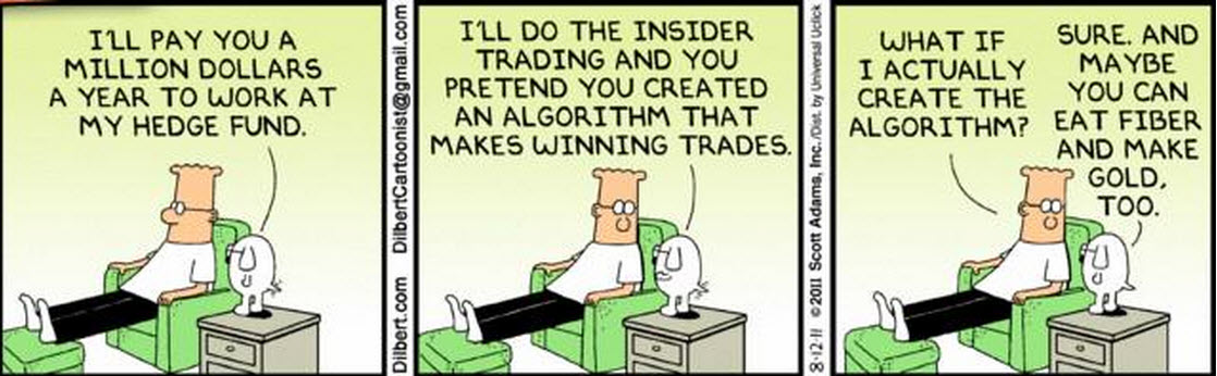
Is there some way we can get the best of both worlds? After all pilots of planes manage it. Autopilot does the boring stuff, but in an emergency humans are able to interpret the situation and act on it much better. I can think of two main routes:

Mechanical system - human override and scaling

Quite a few so called systematic managers seem to operate on the basis of "Yeah, we have all these systems, but we decide when to turn them on and off depending on our judgement". Even firmly committed managers do, occasionally tinker (meddle, risk manage, refit or improve - pick your verb).

Is there a back testable systematic way of switching models on and off that works? If so (and I doubt it) then you're firmly back in the systematic camp.

If not... well it strikes me as just plain stupid that people who know they can't predict market movements think they can predict trading system performance in the same markets.

Discretionary calls - human

This is a much nicer idea. Use your human judgement to decide that Apple is a good bet. Then use a system to decide how much of Apple you should buy, how you should adjust the position as market conditions change, and when you should close. Stick to the system, even when it hurts.

I liked this so much I even put it into my book, where it appears as the the "Semi Automatic Trader" character.

It's also tailor made for the clever and chaotic. Sadly for the committed / useless and useless / chaotic there is nothing that can be done. Use a system, please, for your own sake.

Conclusion

Most humans should trade with systems. Some,who have the skill but not the discipline, can use discretionary trading combined inside a systematic framework. The average human will not be as good as the average computer. Unless you know, for sure, that you'll be well above average as a human trader you should get out your keyboard and start coding.

A story of poor statistical intuition

In continuing my futile quest to raise the level of debate in the quantitative investment community I thought I'd have a go at another clever and very wealthy guy, Cliff Asness, founder of giant fund AQR.

Cliff Asness. There is nothing wrong with his statistical intuition. Or his suit. Nice suit Cliff. (www.bloomberg.com)

To be precise I'm not having a go at Cliff (at some point these billionaires are going to start lawyering up) but at the authors of this specific paper:

www.aqr.com/~/media/files/papers/aqr-alternative-thinking-3q15.pdf

And, to disappoint you further, I'm not really going to 'have a go' at the authors of the paper.

I actually agree completely and wholeheartedly with the sentiments and the conclusions of the paper. I also know that the authors have done and also published other, very good, research which supports the results.

What I have a tiny little problem with is the way that the analysis is presented. More specifically it is about the interaction of a particular human weakness with a particular way of presenting data.

I should also say upfront that this is a problem by no means limited to this paper. It is endemic in the investment industry; and much worse beyond it*. It just so happens that I was sent this paper by an ex-colleague of mine very recently, and it got me a bit riled.

* Here's a great book on the subject of mis representing scientific statistical evidence which is worth reading.

So this post is not a criticism of AQR in particular; and I should reiterate that I have a huge amount of respect for their research and what they do generally.

What does the paper say

If you are too idle to read the paper it looks at the quarterly returns of a bunch of assets and style factors, conditioned on there being a terrible quarter in eithier the bond or equity markets (they also do some stuff with overlapping 12 month returns). For example if you skip to exhibit 1 it shows that for the 10 worst quarters for equities since 1972 fixed income made money in 8 out of 10.

The ex colleague of mine who sent me the paper made the following comment:

"Hello Robert,

Have you seen the paper attached yet? It is interesting that global bonds had a decent performance in the 10 worst quarters for global stocks in 1990-2014, but not the other way around... Trend following seems to have good performance when either stocks or bonds suffer."*

* I've decided to leave my friend anonymous, although he has kindly given permission for me to use this quote.

My first thought was "hmm... yes that is interesting". 

Then after a few minutes I had a second thought:

"Hang on. There are only 10 observations. Is this even statistically significant? "
This was a serious problem. More so because the authors of the paper had also highlighted a key finding, which relates to something I talked about in my last post, trend following. From the paper:

"Trend was on average profitable in all asset classes returns during these equity tail events... As noted, Trend has often performed well in the worst equity quarters... Trend has been a surprisingly good equity tail hedge for more than a century"

I stared at the numbers, but I still couldn't decide whether they were meaningful or not. The underlying problem here is that humans are rubbish at intuitively judging statistical significance - even ones like my friend and I who actually understand the concept.

A bit of small sample statistics

Before proceeding let me briefly explain my outburst on statistical significance. Those who, unlike me, saw immediately whether the results were statistically significant or not can smugly skip ahead.

If we abstract away from the specifics we can reword my friends statement as follows:

"Hypothesis 1: The average return for Bonds, conditional on poor returns for Equities, is positive."
"Hypothesis 2: The average return for Equities, conditional on poor returns for Bonds, is negative"
"Hypothesis 3: The average return for Trend, conditional on poor returns for Equities, is positive"
"Hypothesis 4: The average return for Trend, conditional on poor returns for Bonds, is positive"

The third hypothesis is also one of the main points the author's flagged up.

(By the way, and this is just a small criticism, it might have been more intuitive if the graphs in the paper had been done with Sharpe Ratio units rather than mean returns on the y axis; although do the authors quote the Sharpe Ratio's in the heading. Specifically it would probably have made sense to normalise the quoted returns by the volatility of the full sample.

However I guess what is more intuitive for me might not be to many other people; so I can live with this.)

Notice that in each of the four hypothesis we have an asset we're trying to predict returns for, and another asset that we are conditioning on. We can abstract further to avoid having to model the joint distribution in an explicit way (you can do this of course, but it would take longer to explain):

"Hypothesis 1: The average return for Bonds, in scenario X, is positive."
"Hypothesis 2: The average return for Equities, in scenario Y, is negative"
"Hypothesis 3: The average return for Trend, in scenario X, is positive" 
"Hypothesis 4: The average return for Trend, in scenario Y, is positive"

Obviously Scenario X is bad equity returns, and scenario Y is poor bond returns. The next thing we need to think about is what econometricians would call the data generating process (DGP). This isn't so much where the data is coming from, but where we pretend it's coming from.

We'll treat scenario X and scenario Y individually. Scenario X then consists of a sample of 10 returns drawn from a much larger population which we can't see. Scenario Y is another 10 returns drawn from a different population. The sample mean return for bonds in X is +3.9%; and for equities in Y is -2.7% (from exhibits 1 and 3 respectively). For Trend it's 6.4% for X, and 3% for Y.

I'm also going to assume that the underlying population is Gaussian, with some unknown mean; but with a standard deviation equal to that of the sample standard deviation*; which for bonds X is about 3% a quarter; for equities Y around 5.2% a quarter, and for Trend 7% (X) and 5.3% (Y). This is all a little unrealistic, but again it would be more complicated to do it another way, and it doesn't change the core message.

* Interestingly the full period standard deviation for bonds is 2.6%*** a quarter, equities 6.95%, and trend 5%. Risk seems to be a little higher than normal in equity crisis, but not so much when bonds are selling off.

** derived from annualised figures assuming no auto correlation between quarterly returns

Looking at my hypothesis the null I'm trying to disprove in both cases is that the true population mean return is zero (I could do it other ways, but this is simpler). So let me generate by repeated randomness the distribution of the sample mean statistic for 10 observations, given the estimated standard deviation:

In python:

import numpy as np
import random as rnd
import matplotlib.pyplot as plt

stdev_dict=dict(BOND=3.0, EQUITY=5.2, TRENDX=7, TRENDY=5.3)
sample_mean_dict=dict(EQUITY=-2.7, BOND=3.9, TRENDX=6.4, TRENDY=3.0)

mean=0.0
monte_carlo=100000
sample_size=10

assetname="EQUITY"

stdev=stdev_dict[assetname]
estimate_mean=sample_mean_dict[assetname]

ans=[np.mean([rnd.gauss(mean, stdev) for x in range(sample_size)]) for unused_idx in range(monte_carlo)]
ans.sort()

if assetname in ["TRENDX", "TRENDY", "BOND"]:
    p_value=float(len([x for x in ans if x>estimate_mean]))/monte_carlo
elif assetname=="EQUITY":
    p_value=float(len([x for x in ans if x<estimate_mean]))/monte_carlo
else:
    raise Exception("unknown assetname %s" % assetname)


ax2=plt.gca()
thing=plt.hist(ans, 50)
ax2.get_yaxis().set_visible(False)
plt.title(assetname)
ax2.annotate("%.4f" % p_value, xy=(estimate_mean, 0),xytext=(estimate_mean,max(thing[0])), arrowprops=dict(facecolor='black', shrink=0.05))

plt.show()


First for equities:

Some explanation. The blue histogram shows the distribution of the sample mean, over each of the 100,000 draws of 10 returns. The arrow shows the estimate from exhibit 3, -2.7%. The number above the arrow shows what proportion of the distribution is to the left of our estimate. So there is still a 5.09% chance that average equity returns are zero, conditional on poor bond returns; and we just happen to have drawn a particularly poor set of ten returns in our data.

This result is just shy of significance, using the normal 5% criteria. We can't reject the null hypothesis.

Then for bonds:

Here we have a different story. There is almost no chance that the average return of 3.9% has come from a population with mean zero. We can reject the null. Bonds are a good hedge for equities when things get really bad.

Now for Trend, conditioned on poor equity returns:

This is very significant. Trend is a great equity hedge. Let's see if it is any good for bonds:

Not quite as good, but just creeps into being significant at the 5% level. In summary:

"Hypothesis 1: The average return for Bonds, conditional on poor returns for Equities, is positive." - we can say this is very likely to be true.

"Hypothesis 2: The average return for Equities, conditional on poor returns for Bonds, is negative" - we cannot say if this is true or not.

"Hypothesis 3: The average return for Trend, conditional on poor returns for Equities, is positive" - we can say this is quite likely to be true

"Hypothesis 4: The average return for Trend, conditional on poor returns for Bonds, is positive" - we can say this is probably true


So my friend was mostly right; 3 out of 4 is pretty good. AQR were spot on; in fact the key findings they highlighted were hypothesis 1 and 3, the most highly significant ones. What's more my own personal feelings about allocating to trend following are still justified. However it has taken a fair bit of work to prove this! 

Why we have to tell stories to explain stuff

The crux of the problem is that it's really, really hard to judge what is significant or not in small samples. Most people don't carry around an intuition about these distributions in their heads. But using small samples is quite common in papers like these. The reason is due to a flaw in the human brain, a cognitive bias, narrative fallacy. Or to put it another way we like to hear stories.

If I show you a mass of data points you will probably be thinking 'yeah fascinating. Now what Rob?'. But if I show you a nice graph as in exhibit 1 of the AQR report you'll be thinking '4Q 1987. Black Monday! Ah I remember that / I've read about that (delete depending on age)...'.

1987 crash. Yes children it's true. In the olden days traders wore suits and ties; monitors were really, really big; and the only colour they could display was green (usnews.com)

The information becomes more interesting. Clever researchers know this, and so present information in a way which makes it easier to hang a narrative off.

Why this is bad

This is bad because a story can be both unrepresentative and also statistically meaningless. If I show you a story about an aircraft crashing you are more likely to avoid flying, even if I subsequently show you some dry statistics on the relative safety of different kinds of transport.

A sample of one. (www.cnn.com)

Stories, or if you prefer small samples, can lead us to the wrong judgement*.

* I'm aware that 'you can prove anything with statistics'. However it's true to say that a rigorous analysis of a large sample set, properly presented, is always going to be more meaningful than the inferences a small sample.

Sometimes this is deliberate; as in most tabloid newspapers reporting on medical research. Sometimes it's accidental.

Of course it might be that the small sample is statistically significant, in which case we can draw a conclusion about the general population, as in the case of three out of the four hypothesis we've tested.

However if I see a paper with some small sample results in it, but no indication of significance I don't know if:

• The authors have deliberately shown an unrepresentative and insignificant sample, and the results are wrong
• The authors have got an unrepresentative and insignificant sample by accident, haven't realised it and the conclusions are wrong
• The authors have got a representative sample, but not a significant one. We can't prove the conclusion either way.
• The authors have got a significant and representative sample (the authors may, or may not realise this. I expect the AQR authors did know. These guys aren't sloppy). The authors are correct, but I have no way of knowing this.

Thus there is no way to separate out malicous intent, incompetence and good research which happens to be missing the information needed to understand the significance (as we have here). You need to tell people the values are significant. They won't work it out for themselves (even if they know how, as I do, it's far too much work to generate distributions of sample estimators for every number in every paper I read).

It's for this reason that academic papers are littered with p-values and other statistics (though that doesn't mean you can trust them entirely). I'm not saying that a 'popular finance' paper like this should be festooned with statistical confetti. But a footnote would have been nice.

Conclusion

Don't be afraid of explaining the uncertainty in estimates. Talk about it. Explain it. Let people visualise it. And if you have got significant results, shout about it.

If you're worried that this blog is going to continue in this vein (criticising the research findings of hedge fund billionaires), don't worry. Next time I'll talk about something dull and worthy, like estimating transaction costs; or I'll give you some thrilling python code to read.

But if you're only now following me in the expectation that I'll be writing a post next week about David Shaw's inability to do stochastic calculus, or Ray Dalio's insistence on assuming returns are Gaussian, then I'm sorry you will be disappointed (and if their lawyers are reading, neither of those things are true).

Equilibrium asset pricing models - a quickie (a bit technical)

In my usual daily trawl through FT Alphaville's further reading (worth looking at, registration required but free - it isn't behind the FT's paywall) I came across this little gem.

It's worth reading the full article, but I'd just like to quote a couple of parts:

"Actually I think there has been historically quite a lot of interest in models based on macro factors that would lend themselves relatively naturally to interpretation in terms of equilibrium valuation models. The problem is that they don't tend to work very well empirically... those models just didn't do a good job of explaining a substantial fraction of asset returns... Plus they usually seem to have unobservable or hard-to-observe components. For example, any model of interest rates is going to have to have some place for a market price of interest rate risk.... Even a small error in that estimate is going to produce a huge discrepancy to observed yields."

To be clear we're talking about models of the form P = f (a,b,c....) where P is the 'correct' asset price, and a,b,c are factors like for example the market price of interest rate risk and other such. To make these models work you also need to know the factor loadings; if the model was linear these loadings would just be the coefficients on the various factors in a pricing equation.

If this sounds like mumbo jumbo, bear in mind you probably already know about one such model, which is the CAPM (if you don't know what the CAPM is then it's still going to sound like mumbo jumbo and this post probably isn't for you). In the CAPM the factor is the market return and the loadings is the much maligned beta (covariance with the market). The CAPM equation is specified in excess returns rather than expected values, but it's easy to switch between the two when we note that the correct value is equal to todays price plus the expected return. If we add in the expected speed of reversion to the correct value then we can make the two approaches equivalent.

Now I've spent a fair bit of my own time in the past messing around with these models, and I have a few thoughts and ideas to share. To make this post more tractable I'll refer to a specific examples: where we are trying to estimate the equity risk premium.

Choice of factor

There is an unfortunate habit in the literature of these models to choose factors which have nice economic meaning, regardless of whether they are observable. So for example in the equity risk premium world it usually makes more sense to use expected real interest rates. However it's difficult to get inflation expectations for some long horizon. In some countries you can use inflation linked securities, but biases mean it's not easy to extract inflation expectations from them. Survey measures are better, but will rarely go back  (for a longer and better discussion of this see Expected Returns).

It's tempting to fall back on creating your own model to forecast inflation. A reasonable model would include an equilibrium (based on a moving average of inflation), a rate of change (recent changes in inflation) and survey and asset price measures if available. Note however we've just exploded the number of coefficients we have to estimate. Also if the model is to forecast a long time in the future (say 20 years) it's going to consume a lot of data history, and waste the last two decades worth.

An unpleasant class of models is where the loadings are specified, and you find the factors. This is done in parts of the bond pricing literature. One of the few nice things about the macro factor models is that the factors have some kind of meaning. But rather than have intuitive interest rate factors like the level of rates, and the steepness of the curve, we have a factor which is based on a weird function of forward rates.

Reversion to equilibrium

An obvious point is that these models are no good if they don't get the equilibrium value correct. As the quote notes a slight difference in the equilibrium can make a big difference. For example the equilibrium PE ratio of stocks (which we can extract from the equity risk premium) under one model might be 20, and with slightly different assumptions it might be 15. Give the normal range of stock PE ratios this will make a huge difference to performance.

source: investopedia

The opposition - kitchen sink

You can think of a macro factor model as a big bunch of variables in a regression; on some of which the coefficients or relative coefficients are specified (like the current real interest rate is the nominal interest rate minus current inflation); and others (the loadings) which we have to estimate.

Given all the caveats above you might conclude the best approach is to just throw all the observable factors you have into a giant kitchen sink regression and let them fight it out. So rather than trying to cobble together an inflation forecasting mini model as above, you just chuck the underlying observable variables into the regression with everything else.

But the big advantage of having some pre-existing structure in your data is it reduces the degrees of freedom, and if you are right about the structure will give you a more robust model.

(You could also take a Bayesian view that you think your imposed structure is correct, unless proven statistically false).

The opposition - simple mean reversion

There is an even simpler method, which is to do a simple mean reversion model on one or more valuation factors. So in stocks you would just take the history of PE ratios, and then take some kind of slow moving average to measure the equilibrium. If the PE dips below that equilibrium then you buy; otherwise you sell.

Mild improvements can be made to this by incorporating more sensible variables, as is done in the CAPE model with real earnings, as long as you don't put yourself into a position when you have to start estimating coefficients again.

Mean reversion isn't, usually, strong enough

These macro models should have an advantage over a kitchen sink approach where the same kind and number of underlying variables are regressed without any structure being imposed. However they're unlikely to beat a relatively simple mean reverting model. Worst still all such mean reverting models only perform well at relatively slow time scales, useless to any active investor.

If for example you are forecasting at a horizon of a few months, and you add a 'momentum' factor to your model, you'll find it dominates all your other predictive variables.

What kind of valuation model works at sensible time scales?* No, not a macro model but a micro, relative value, model with asset specific factors in it. In this case we don't need to worry if the equilibrium is correct or not; it's implicit in the fact that we have no net exposure, only relative value bets.

* though having said that relative momentum is also important in these kinds of models.

Good at telling you where you are... not where you're going

I have similar feelings about these kinds of models as I do about "big data" (bear with me). Big data, it strikes me, is very good at modelling the current behaviour of for example spending by loyalty card shoppers*. Each of those shoppers is relatively similar (they all go to the same supermarket for a start), and importantly they are not interacting with each other, nor do their shopping habits change much when for example the US non farm release comes out. Unless their behaviour changes radically, which it tends not to, we can make some reasonable predictions about how they will behave.

However big data and market forecasting is more difficult. The prices are a result of a large number of relatively heterogenous participants interacting, and reacting to exogenous news and shocks, in a way that supermarket shoppers hardly do. At best you can overfit to the extreme and tell some interesting stories. Just don't try using it to trade.

Similarly well specified macro models can tell you some very interesting stories about the past. So it's possible to disaggregate the equity risk premium (without incidentally needing to estimate any coefficients), and conclude that much of the excess return of equities in the last 40 years is due to a secular fall in inflation.

The only useful prediction I can make out of that is that equity returns are likely to be lower in the future. That's useful, but it barely qualifies as a forecast and its no use whatsoever for any kind of dynamic trading.

 

Conclusion

It's fun playing with macro models, and they're intellectually interesting, but they have no place in the armory of any investor or trader.