The US QE2 programme began in November 2010, and it finished in late 2014. We knew that QE was keeping interest rates relatively low and stable. We knew at some point it would end, and interest rates would rise.
(I'm writing this as a trader rather than an economist, and the fine distinction between the effects of Fed Fund rate rises and the slowing or reversing of asset purchases do not concern us here)
Our number one concern was how our models would react when this event happened. Would our strategies cope, or would they be badly underwater? Given that the QE unwind is still underway this is still very much a live discussion.
The problem here is one of meta-prediction. We aren't trying to predict interest rates, or the returns of assets like US bond futures; we already have our underlying trading strategies for that: momentum, carry, and perhaps a few other bits and pieces. Instead we're trying to make predictions about the returns of the trading strategies. Does momentum do better in particular regimes? Can we identify when carry is likely to under perform? If so we can reallocate our risk capital into the most favourable place. Essentially this is a problem of factor timing. Like Cliff says, factor timing is hard. But let's try anyway.
Some messy python code using pysystemtrade is here
An idiots guide to meta-prediction
Meta-prediction requires two important ingredients:
- A strategy, or strategies, whose returns we can back test historically.
- A conditioning variable to identify a particular regime (for simplicity I'm assuming that regimes are discrete rather than continuous here)
Assuming we have these two ingredients our job is easy: partition our historic strategy returns by regime, and test whether there is any difference in strategy performance. We then find the regime that is closest to what we expect to happen next, and determine if our strategy will do better or worse than average.
Choice of strategies
To keep things relatively simple I'm going to use the four core trading rule variations from chapter 15 of my first book: Carry, and 3 variations of momentum - fast, medium, slow (moving average crossovers with speeds 16/64, 32/128, 64/256).
The choice of instruments is more interesting. Obviously we'd see clearer effects if we looked at Eurodollar futures and US bonds; even clearer if we aligned the instrument with the conditioning variable (eg using a 2 year interest rate to see what happens with 2 year bond futures). Of course there are likely to be spillover effects into other bonds, and possibly into other asset classes (the fear of rising interest rates appears to have been one of the causes of the recent sharp sell off in equities). To keep things simple in this post I'm mostly going to look only at the following US interest rate related futures:
- Eurodollar (traded approximately 3 years out on the curve)
- US 5 year
- US 10 year
- US 20 year (I don't actually trade this but I have the data so why not)
(The US 2 year bond future has insufficient data, so I'm ignoring that. Also I'm focusing purely on US QE in this post. Finally I'm ignoring the possibility of extrapolating from the earlier Japanese QE experiment, and seeing what lessons this would have for the US)
Conditioning variable
To be useful conditioning variables need to have some key properties:
- Quantifiable
- Present in history
- Meaningful historic variation
- Reasonably distributed
- Ex-Ante
'Quantifiable' is, I hope, self explanatory to the average reader of this blog. By 'present in history' I mean that we have a long historical record of the variable. QE fails badly on this measure - we've never had QE in the US before.
The OIS - LIBOR spread is an example of a spread that didn't have meaningful variation prior to 2007. It also isn't 'reasonably distributed' - the distribution prior to 2007 is completely different from what followed.
A key part of making meta predictions is to use an ex-ante rather than an ex-post variable. Official US recessions are an example of an ex-post variable - the official announcement is made around a year after each change in regime. Ex-post analysis is interesting, but useless when it comes to making predictions.
Given that QE itself is flawed, what is a variable that is a good QE proxy and satisfies all of the above conditions? A naive description of the effect of QE reversing would be something like this “Interest rates are low, but have started rising”. The level and change in interest rates would seem to be appropriate variables. To keep things ex-ante we'd need to ensure we measured the level at the start of the period (if we're using daily returns this just means lagging the rate by a day). Similarly the change needs to be up to the start of the period. Let's use the change in the previous 12 months up to the start of the return period.
Which interest rate should we use? The Fed Funds rate is an obvious one. But given we're concerned with QE, which was designed to make bond yields lower, I think we should focus on government bond yields. The average maturity of US debt is relatively short, around 4-6 years. So I'm going to use this 5 year constant maturity bond rate.
Note: the results are similar with the Fed Funds Rate
Here is the interest rate level:
 |
| US 5 year constant maturity rate (https://www.quandl.com/data/FRED/DGS5-5-Year-Treasury-Constant-Maturity-Rate) |
I'm not super happy with this variable. If we condition on rate level we'll probably end up partitioning on time: pre 1995 and post 1995. I'm not sure how meaningful the results from that will be. Here is the 12 month change:
 |
| Rolling 12 month change in 5 year US interest rates |
The amplitude of changes is clearly higher when interest rates are higher; but I'd argue that a 100bp increase is far more significant now than it was back in the early 1980s. However the problem isn't as serious as for the level: this is mostly a reasonably stationary series.
To cope with this I'm going to apply a normalisation to the level: I will divide by the rolling 20 year average of the interest rate. Since interest rate cycles normally last about 10 years this will give us an indication of where we are in the rate cycle; a far more useful conditioning variable.
Here is the normalised level:

Much nicer. After adjustment you can see that interest rates are clearly in a higher part of the cycle than the unadjusted rate would suggest. Here is the normalised change:

- Normalised interest rate level (divided by 10 year average)
- Normalised interest rate change over last 12 months
Some naive results
Interest rate levels (normalised)
To kick things off here is the account curve for Eurodollar carry, coloured to show the two regimes for normalised interest rate levels.
 |
| Carry account curve for Eurodollar futures, conditional on normalised interest rate regime |
Notice how we are currently in a 'high' interest rate environment, and that apart from the early 1980's returns look to have been better when rates are low. An open question here is whether we should use return or Sharpe Ratio. It looks like the volatility might be different in the high interest rate environment. I'm going to use Sharpe Ratio, but you should bear this in mind.
Here are the results for Eurodollar futures across different trading rules:
 |
| Sharpe Ratio for Eurodollar futures across trading rule variations, conditioned on normalised 5 year rates |
The 'low' rate environment here is a normalised range of 0.15 to 0.71; whilst for 'high' it's from 0.71 to 1.57 (these buckets are divided at the median value of the conditioning variable). The rate is currently over 1.0; so at least on a normalised basis we're actually in a 'high' rate environment (in contrast in 2013 just before the 'taper tantrum' the adjusted rate was at an all time low of 0.15).
There seems to be some weak evidence that 'high' is better than low, especially for momentum.
Here are the results for the bond futures:
|
 |
| Sharpe Ratio for 5 year futures across trading rule variations, conditioned on normalised 5 year rates |
 |
| Sharpe Ratio for 10 year futures across trading rule variations, conditioned on normalised 5 year rates |
 |
| Sharpe Ratio for 20 year futures across trading rule variations, conditioned on normalised 5 year rates |
These are very mixed results. Because of this, and because the normalisation makes things slightly tricky, I don't think there is anything worth pursuing here.
Interest rate changes (normalised)
Now let's move on to looking at interest rate changes. We'll start with Eurodollar, and then move up through the tenors.
Here is the account curve for Eurodollar and the slowest momentum rule, hacked to show the different regimes:
 |
| Carry account curve for Eurodollar futures, conditional on normalised interest rate change regime |
Notice how we're currently in a rising regime (orange), and how good performance is almost entirely confined to falling rate regimes (blue). Notice also that the trading rule reduces it's volatility when we lose money; this is a classic pattern for trend following. This also means that using conditional Sharpe Ratio is perhaps a little unfair; the absolute losses will be smaller when rates are rising even if the SR looks really bad.
Anyway, do these results hold across other trading rules?
 |
| Eurodollar futures, performance of trading rules conditioned on normalised rate changes |
'Fall' means the normalised interest rate change was in the range -0.48 to -0.04 over the previous 12 months before the relevant day. 'Rise' means the rate changed was in the range -0.04 to +0.40. The reason for this skew in buckets is of course that interest rates have mostly fallen in the period we're using, and the normalisation doesn't quite correct for this. Changing the buckets so that they cover a strictly negative and positive range won't affect the results.
The current 12 month change in rates is +0.26, so we're solidly in the rising interest rate environment here.
That is a very consistent pattern but let's see if that is repeated across other instruments:
 |
| US 5 year bond futures, performance of trading rules conditioned on normalised rate changes |
 |
| US 10 year bond futures, performance of trading rules conditioned on normalised rate changes |
 |
| US 20 year bond futures, performance of trading rules conditioned on normalised rate changes |
There is a very consistent pattern here: recent rises in interest rates are bad news for carry, and really bad news for momentum (especially the slowest kind). Here is a nice summary chart that shows what happens if we lump all the different futures into a single portfolio (equally weighted):
 |
| Portfolio of US bond & rate futures, performance of trading rules conditioned on normalised rate changes |
This sort of makes sense: if rates are rising then the net effect of still positive carry plus negative price movements can lead to a 'choppy' total return series; choppy prices are seriously bad news for any kind of trend following; if carry stays long it will benefit from positive total return even if it's much much smaller than what we see in falling rate environments.
What about across portfolios? Here is the performance of each instrument, after applying some sensible forecast weights: system.config.forecast_weights = dict(ewmac16_64 = 0.2, ewmac32_128 = 0.2, ewmac64_256 = 0.2, carry=0.4)
 |
| Portfolio of trading rules, Sharpe Ratio across instruments, conditioned on normalised rate changes |
Focusing on the pattern of Sharpe Ratios it looks like you might want to up your allocation to US 5 years, but reduce fixed income generally.
Now we may have done a little data mining to get to this point, but blimey! That is one strong result! Consistently falling Sharpe Ratio as we move from a regime of recently falling rates to one of recently rising. It appears to be a very convincing null points for fixed income momentum and carry in the current regime.
Some less naive results
The results above look compelling, and no doubt have many people working in CTAs rushing to deallocate from fixed income momentum as we speak. If we were working for the sell side, where our job was to generate flow rather than do proper research, we'd probably stop there.
But they miss out on an important point: we're only seeing the average conditional return, not the distribution of conditional returns. This is important because the average doesn't tell us how significant the difference is between the returns we're seeing. More specifically what we want is the sampling distribution of the Sharpe Ratio estimate.
We know from Andrew Lo that for i.i.d. returns this has a standard deviation of root(1+.5SR^2).
(For non-normal distributions check out Opdyke)
Rather than mucking about with fancy formula that aren't quite accurate anyway let's bootstrap the relevant distributions. To avoid plot overload I'm going to do these for each trading rule variation individually, for a portfolio of instruments.
Here's the plot for carry
 |
| Histogram of sampling estimate for SR, across instruments, for carry rule, conditioned on normalised yield change |
There is clearly a serious difference between the performance here. The p-value for a t-test of the performance across these two regimes comes in at just over 1%.
Legend key: Range of conditioning variable, Mean Sharpe Ratio estimate, Independent t-Test p-value for comparing with the worst Sharpe Ratio
The results for other trading rules are equally strong or stronger, so to cut to the chase here is a plot for the entire portfolio of fixed income trading rules and instruments:
 |
| Histogram of sampling estimate for SR, across instruments, for all rules, conditioned on normalised yield change |
The t-test p-value is pretty significant here, again well under 5%. It turns out that there is a pretty substantial difference in fixed income strategy performance across different interest rate regimes.
By the way although the result is significant, it isn't as clear cut as the p-value above might lead you to believe. If we cut our data into finer regimes then we get the following Sharpe Ratios:
 |
| Average Sharpe Ratio for portfolio of all fixed income instruments and trading rules conditional on normalised interest rate regime |
Due to the way the regimes are created each bucket as an identical length of return history, but the rate regimes may be of different widths.
A few more experiments
Lest we be accused of p-hacking, here is the result for the unadjusted yield change:
 |
| Histogram of sampling estimate for SR, across fixed income instruments, for all rules, conditioned on raw yield change |
If anything the results here are more significant than for the normalised yield change. For reference the current 12 month trailing interest rate rise is +0.64%; so we do fall in the orange distribution, but only just. The results here aren't quite as relevant for current meta-predictions than those for the normalised change.
Fixed income is buried, but what about the rest of our CTA portfolio? Should we try a different asset class? Here are the results for S&P 500:
 |
| Histogram of sampling estimate for SR, S&P 500 futures, for all rules, conditioned on raw yield change |
Finally here are the results for a couple of long only portfolios (i.e. we're now making predictions not meta-predictions). First long only equally weighted for all four of our fixed income instruments (actually these are inverse vol weighted, not equal weighted):
 |
| Histogram of sampling estimate for SR, across fixed income instruments, for long only portfolio, conditioned on adjusted yield change |
The results here make sense on one level, but not on another. This plot shows us that if interest rates have recently been rising then we should expect to do relatively badly from fixed income (although the p-value isn't that significant). Another way of putting that is that momentum works: if interest rates have been rising then total return from long only bond portfolios won't be that great (although this measure of momentum is the 12 month change in a single yield, rather than a moving average crossover on the adjusted price of whatever). However we already know that slow momentum is best avoided in fixed income when yields have been rising.
And here is long only S&P 500:
 |
| Histogram of sampling estimate for SR, S&P 500 futures as long only portfolio, conditioned on adjusted yield change |
It looks like rising rate environments are slightly better for stocks (due to higher economic confidence?) but again this is a long way from being significant. Interesting though and possibly the source of a trading rule idea for stock index prediction.
Summary: what should we do?
Here is a quick summary of the Sharpe Ratios that we've seen so far for each normalised interest rate change regime, plus the p-values when comparing the two regimes.
Falling Rising P-value
SP500 long 0.04 0.45 28.00%
FI long 0.9 0.44 13.50%
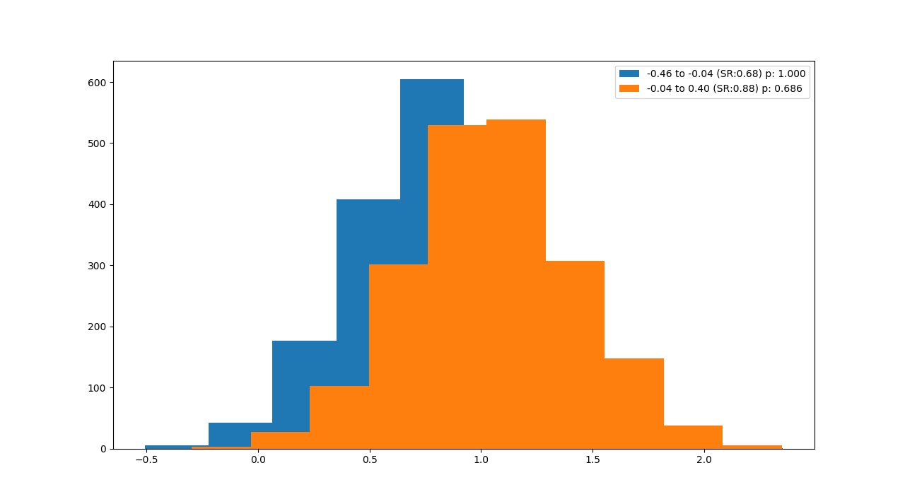
SP 500 CTA 0.68 0.88 69.00%
FI CTA 0.91 0.18 2.00%
EDOLLAR CTA 0.96 0.18 2.20%
US5 CTA 0.84 0.36 18.20%
US10 CTA 0.86 0.25 6.50%
US20 CTA 0.58 0.12 14.00%
FI carry 0.92 0.14 1.20%
FI slow mom 0.7 -0.25 0.20%
FI med mom 0.64 -0.02 2.50%
FI fast mom 0.66 0.10 7.30%
It looks like in a rising interest rate environment you should make the following portfolio adjustments:
- Long only: Shift to stocks and out of bonds (although bonds still do about as well as stocks in a rising rate environment - it's just that they're not doing as well as when rates are falling and stock performance is flat)
- CTA vs long only: Perhaps slightly reduce your overall CTA exposure, but not by much (stock CTA strategies actually do a little better, and CTA returns won't be much lower if managers deallocate from fixed income)
- CTA asset allocation: Shift out of fixed income and into other asset classes.
- CTA fixed income instrument weighting: You might want to slightly overweight 5 years at the expense of other tenors
- CTA fixed income forecast allocation: You might want to slightly overweight faster momentum at the expense of slower momentum (the slow momentum loses out most when we don't get a tailwind of general reductions in yield). On a relative basis carry holds up reasonably well versus momentum.
By the way 'shift' doesn't imply a complete reallocation. I'd be wary of changing my weights by more than a factor of 0.5 / 1.5, even with p-values of 2% or less. So for example if your CTA portfolio is 30% in fixed income; then the largest reduction I'd countenance would be to shift it to 15% in fixed income.
Concluding thoughts
I will be honest - I was surprised by these results - and I didn't set out to find them (always a risk with any piece of research). It's unusual to find meta-predictions that work. Out of loyalty to CTAs generally, and to fixed income specifically, I was rather hoping to find no significant effects.
Have I discovered a holy grail of factor timing? It depends what you mean by factor timing. I haven't shown that we can predict when momentum or carry can do well relative to buy and hold for a given asset class. All I've confirmed is that rising interest rates are not ideal for fixed income, and the results show that is true not only for long only, but also for most strategies that you might care to mention.
But if 'bond momentum' and 'bond carry' are factors, then sure I've found a pretty good predictor of when it does or doesn't work: recent rises in interest rates. Although remember from before that momentum will partially turn itself off when it is losing money, due to weaker signals as you'd expect to get when rates are rising.
I probably won't personally do anything with these results because it's an extra layer of complexity (and I haven't formally back-tested using interest rate changes to alter weightings, which means I haven't accounted for switching costs; plus there is the question as to how we approach say other countries like Germany where I don't have enough data to prove whether this works).
But they are still interesting food for thought.