Showing posts with label skew. Show all posts

Monday, 5 May 2025

Can I build a scalping bot? A blogpost with numerous double digit SR

 I did post recently, from which I shall now quote:

Two minute to 30 minute horizon: Mean reversion works, and is most effective at the 4-8 minute horizon from a predictive perspective; although from a Sharpe Ratio angle it's likely the benefits of speeding up to a two minute trade window would overcome the slight loss in predictability. There is no possibility that you would be able to overcome trading costs unless you were passively filled, with all that implies... Automating trading strategies at this latency - as you would inevitably want to do - requires some careful handling (although I guess consistently profitable manual scalpers do exist that aren't just roleplaying instagram content creators, I've never met one). Fast mean reversion is also of course a negatively skewed strategy so you will need deep pockets to cope with sharp drawdowns. Trade mean reversion but proceed with great care.

Am I the only person who read that and thought.... well if anyone can build an automated scalping bot... surely I can? 


To be precise something with a horizon of somewhere around the 4-8 minute mark, but we'd happily go a bit slower (though not too much, lest we hit the dreaded region of mean reversion), or even a bit quicker.

In fact I already have the technology to build one (at least in futures). There's a piece of code in my open source trading system called the (order) stack handler. This code exists to manage the execution of my trades, and implements my simple trading algo, which means it can do stuff like this: 

- get streaming prices from interactive brokers

- place, modify and cancel orders, and check their status with IB

- get fills and write them to a database so I can keep track of performance

- work out my current position and check it is synched with IB

I'll need to do a little extra coding and configuration. For example, I will probably inherit from this class to create my little scalping bot. I will also want to partition my trading universe into the scalped instruments, and the rest of my portfolio (it would be too risky to do both on a given market; and my dynamic optimisation means removing a few instruments from my main system won't cause too much of a headache).

All that leaves then is the "easy" job of creating the actual algo that this bot will run... and doing so profitably.

Some messy python (no psystemtrade required), here, and an sketchy implementation in psystemtrade here.


Some initial thoughts

I'm going to begin with a bit of a brain dump:

So the basic idea is that we start the day flat, and from the current price we set symmetric up and down bracket limit orders. To simplify things, we'll assume those orders are for a fixed number of contracts (to be determined); most likely one but could be more. Also to be determined are the width of those limit orders.

Unlike the (now discredited) slower mean reversion strategy in my fourth book, we won't use any kind of slow trend overlay here. We're going to be trading so darn quick that the underlying trend will be completely irrelevant. That means we're going to need some kind of stop loss. 

If I describe my scalper as a state machine then, it will have a number of states. Let's first assume we make money on a buy.

A: Start: no positions or orders

- Place initial bracket order

B: Ready: buy limit and sell limit

- Buy limit order taken out

C: Long and unprotected: (existing) sell limit order at a profit

- Place sell stop loss below current level

D: Long and protected: (existing) sell limit order at a profit (higher) and sell stop loss order (lower)

- Hit sell limit profit order

E: Flat and unbalanced: sell stop loss order

- Cancel sell stop loss order

A: No positions or orders

Or if you prefer a nice picture:


Lines are orders, black is price, then green because we are long, then black again when we are flat. Red lines are sell order, dotted line is stop loss, green line is buy order.

What happens next: is we reset, and place bracket orders around the current price which is assumed to be the current equilibrium price. Note: if we didn't assume it was the current equilibrium we would have the opportunity to leave our stop loss orders in place. But that also assumes we're going to use explicit stops, which is a design decision to leave for now.

The other profitable path we can take is:

B: Ready: buy limit and sell limit

- Sell limit order taken out

F: Short and unprotected: (existing) buy limit order at a profit

- Place buy stop loss above current level

G: Short and protected: (existing) buy limit order at a profit (lower) and buy stop loss order (higher)

- Hit buy limit profit order

H: Flat and unbalanced: buy stop loss order

- Cancel buy stop loss order

A: No positions or orders


Now what if things go wrong?

D: Long and protected: (existing) sell limit order at a profit (higher) and sell stop loss order (lower)

- Hit sell limit stop loss

J: Flat and unbalanced: sell limit order

- Cancel sell limit order

A: No positions or orders


Alternatively:

G: Short and protected: (existing) buy limit order at a profit (lower) and buy stop loss order (higher)

- Hit buy stop loss limit

K: Flat and unbalanced: buy limit order

- Cancel buy limit order

A: No positions or orders


That's a neat ten states to consider. Of course with faster trading there is the opportunity for async events which will effectively result in some other states occuring, but we'll return to that later. Finally, we're probably going to want to have a 'soft close' time before the end of the day beyond which we wouldn't reopen new positions, and then a 'hard close' time when we would close our existing position irrespective of p&l.

It's clear that the profitability, risk, and the average holding period of this bad boy are going to depend on what proportion of our trades are profitable, and hence on some parameters we need to set:

- position size

- initial bracket width

- distance to stop loss


... some numbers we need to know:

- contract multiplier and FX

- commissions and exchange fees

- the cost of cancelling orders 


... and also on on some values we need to estimate:

- volatility (we'd probably need a short warm up period to establish what that is)

- likely autocorrelation in prices

Note: We're also going to have to consider tick size, which we need to round our limit orders, but also in the limit will result in a minimum bracket width of two ticks (assuming that would still be a profitable thing to do).

Further possible refinements to the system could be to avoid trading if volatility is very high, or is in a period of adjustment to a higher level (which depending on time scale can basically mean the same thing). We could also throw in a daily stop loss on the scalper, if it loses more than X we stop for the day as we're just 'not feeling it'.

Another implementation detail that springs to mind is how we handle futures rolls; since we hope to end the day flat this should be quite easy; we just need to make sure any rolls are done overnight and not trade if the system is in any kind of roll state (see 'tactics' chapter in AFTS and doc here).


Living in a world of OHLC

Now as you know I'm not a big fan of using OHLC bars in my trading strategies -  I normally just use close prices. I associate using OHLC prices and creating candle stick charts with the sort of people who think Fibbonaci is a useful trading strategy, rather than the in house restaurant at a london accountants office

However OHLC do have something useful to gift us, which is the concept of the likely trading range over a given time period (the top and the bottom of a candle). 

Let's call that range R, and it's simply the difference between the highest and lowest prices over some time horizon H (to be determined). We can look at the most recent time bucket, or take an average over multiple periods (a stable R could be a good indication of stable volatility which is a good thing for this strategy). So for example if we're looking at '5 minute bars' (I'll be honest it takes an effort to use this kind of language and not throw up), then we could look at the height of the last bar, or take a (weighted?) average over the last N bars.

Now to set our initial bracket limit orders. We're going to set them at (R/2)*F above and below the current price. Note that if F=1, we'll set a bracket range which is equal to R. Given we're assuming that R is constant and represents the expected trading range, we're probably not going to want to set F>=1.  Smaller values of F mean we are capturing less of the spread, but we're exposed for less time. Note that setting a smaller F is equivalent to trading the same F on a smaller R, which would be a shorter horizon. So reducing F just does the same thing as reducing R. For simplicity then, we can set F to be some fixed value. I'm going to use F=0.75.

Finally, what about our stop losses? It probably makes sense to also scale them against R. Note that if we are putting on a stop loss we must already have a position on, which means the price has already moved by (R/2)*F. The remaining price "left" in the range is going to be (R/2)*(1-F); to put it another way versus the original 'starting' price we could set our stop loss at (R/2) on the appropriate side if we wanted to stop out at the extremes of the range. But maybe we want to allow ourselves some wriggle room, or set a stop closer to our original entry point. Let's set our stop at (R/2)*K from the original price, where K>F. 

Note this means our (theoretical!!!) max loss on any trade is going to be (R/2)*(K-F). For example, if F=0.75 and K=1.25 (so we place our stops at the extreme of the range), then the most we can lose if we hit our stop precisely is R/4.


Back of the envelople p&l

We're now in a position to work out precisely what our p&l will be on winning trades, and roughly (because stop loss) on losing trades. Let's ignore currency effects and set the multiplier of the future to be M (the $ or otherwise value of a 1 point price move). Let's set commission to C and also assume that it costs C to cancel a trade (the guidance on trade cancelling cost in interactive brokers docs is vague, so best to be conservative). In fact it makes more sense to express C as a proportion of M, c.
Finally we assume we're going to use an explicit stop loss order rather than implicit which means paying a cancellation charge.

win, W = R*F*M - 3C = R*F*M - 3Mc = M(R*F - 3c)
loss, L = -(K-F)*M*R/2 - 3C = -M[(K-F)*R/2 + 3c)

I always prefer concrete examples. For the SPY micro, M=$5, C=$0.25, c=0.05 and let's assume for now that R=10. I'll also assume we stick to F=0.75 and K = 1.25. So our expected win is:

W = $5 * (10*0.75 - 3*0.05) = $36.75
L = -5*[(1.25 - 0.75)*10/2 +3*0.05] = -$13.25

Note that in the absence of transaction costs the ratio of W to L would be equal to 2F / (F-K) which in this case is equal to 3. Note also that the breakeven probability of a win for this to be a profitable system is L / (L-W) which would be 0.25 without costs, but actually comes out at around 0.265 with costs.

We can see that setting K will change the character of our trading system. The system above is likely to be quite positive skew (breakeven probability). If we were to make K smaller, then we'd have more wins but they are likely to be smaller, and we'd get closer to negative skew.


Introducing the speed limit

Readers of my books will know that I am keen on something called the 'speed limit'; the idea that we shouldn't pay too much of our expected return on costs. I recommend an absolute maximum of 1/3 of returns paid out on costs; in practice eg for my normal trading strategy I pay about 1% a year and hope to earn at least ten times on that.

On the same logic, I'm not sure I'd be especially happy with a strategy where I have to pay up half my profits in costs even on a winning trade. Let's suppose the fraction of gross profit I am happy to pay is L, then:

3Mc / R*F*M = L

R = 3c / LF

For example, if L was 0.1 (we only want to pay 10% of our costs), then the minimum R for F=0.75 on the S&P 500 with c=0.05 would be 3*.05 / (0.1 * 0.75) = 2

In practice this will put a floor on the horizon chosen to estimate R; if H is too short then R won't be big enough. The more volatile the market is, the shorter the horizon will be when R is sufficiently large. However we would want to be wary of a longer horizon, since that would push us towards a holding period where autocorrelation is likely to turn against us (getting up towards 30 minutes).

But as we will see later, this crude method significantly understimates the impact of costs as it ignores the cost of losing trades. In practice we can't really use the speed limit idea here.


Random thought: Setting H or setting R?

We can imagine two ways of running this system:

- We set R to be some fixed value. The trading horizon would then be implicit depending on the volatility of the market. Higher vol, shorter horizon. We might want to set some limits on the horizon (this implies we'll need some sensitivity analysis on the relationship between horizon and the ratio of R and vol). For example, if we go below a two minute horizon we're probably pushing the latency possibilities of the python/ib_insyc/IB execution stack, as well as going beyond the horizon analysed in the arvix paper. If we go above a fifteen minute horizon, we're probably going to lose mean reversion again as in the arvix paper. 
- We set the horizon H at some fixed value, and estimate R. We might want to set some limits on R - for example the speed limit mentioned above would put a lower limit on R. 

In practice we can mix these approaches; for example estimating R at a given horizon at the start of each day (perhaps using yesterdays data, or a warm up period), and then keeping it fixed throughout the day; or maybe re-estimating once or twice intraday. We can also at this point perhaps do some optimisation on the best possible value of H; the period when we see the best autocorrelation.

Simulation

Right, shall we simulate this bad boy? Notice I don't say backtest. I don't have the data to backtest this. I'm going to assume, initially, very benign normal distribution returns that - less benign - has no autocorrelation.

Initially I'm going to use iid returns, which is conservative (because no autocorrelation) but also aggresive (no jumps or gaps in prices, or changes in volatility during the day). I'm also going to use zero costs and cancellation fees, and optimistically assume stop losses are filled at their given level. We're just going to try and get a feel for how changing the horizon, and K affect return distribution. I'm going to re-estimate R throughout the day with a fixed horizon, but given the underlying distribution is random this won't make a huge amount of difference.

The distribution is set up to look a bit like the S&P 500 micro future; I assume 20% annualised daily vol and then scale that down to an 8 hour day (so no overnight vol). That equates to 71.25 units of price of daily vol, assuming the current index level of ~5700. I will simulate one day of ten second price ticks, do this a bunch of times, and then see what happens. The other parameters are those for the S&P micro: contract multiplier $5, tick size $0.25, and I also use a single contract when trading.

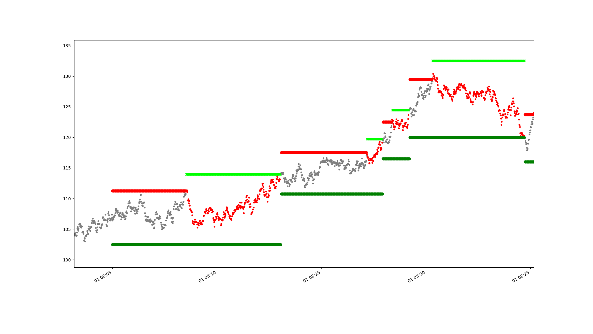
The simulations can be used to produce pretty plots like this which show what is going on quite nicely:

The price is in grey, or red when we are short, or green if long. The horizontal dark red and green lines are the initial take profit bracket orders. You can see we hit one early on and go short. The light green line is a buy stop loss (there are no sell stop losses in this plot as we're only ever short). You can see we hit that, so our initial trade fails. We then get two short lived losing trades, followed by a profitable trade near the end of the period when the price retraces from the red bracket entry down to the green take profit line.

Here's a distribution of 5000 days of simulation with a 5 minute horizon, and K=1.25 (with F=0.75):


Well it loses money, which isn't great. The loss is 0.4 Units of the daily risk on one contract (daily vol 71.25 multiplied by multiplier $5). And that's with zero costs and optimistic fills remember. Although there is a small point to make, which is that this isn't a true order book simulator. I only simulate a single price to avoid the complexity of modelling order arrival. In reality we'd gain a little bit from having limit orders in place in a situation where the mid price gets near but doesn't touch the limit order. Basically we can 'earn' the bid-ask bounce. 

The distribution of daily returns is almost perfectly symettrical, obviously that wouldn't be true of the trade by trade distribution.

What happens if we set a tighter stop, say K=0.85?

Now we're seeing profits (0.36 daily risk units) AND some nice positive skew on the daily returns (which have a much lower standard deviation of about 0.40 daily risk units). Costs are likely to be higher though, and we'll check that shortly. Note we have a daily SR approaching 1.... which is obviously bonkers- it annualises to nearly 15!!! Incredible bearing in mind there is no autocorrelation in the price series at all here. But of course, no costs.

What happens if we increase the estimate period for R to 600 seconds (10 minutes), again with K=0.85:

Skew improves but returns don't. Of course, costs are likely to fall with a longer horizon.


An analysis of R and horizon

Bearing in mind we know what the vol of this market is (71.25 price units per day), how does the R measured at different horizons compare to that daily vol? Note this isn't affected by the stoploss or costs.

At 60 seconds, average R is 4.6, in daily vol units: 0.065
At 120 seconds, .... R in vol units: 0.10
At 240 seconds, ...  R in vol units: 0.15
At 360 seconds, ...  R in vol units: 0.19
At 480 seconds, ...  R in vol units: 0.22
At 600 seconds, ... R in vol units: 0.25
At 900 seconds, ... R in vol units: 0.31

This doesn't quite grow at sqrt(T) eg T^0.5, but at something like T^0.59.

Footnote: even the smallest value of R here is greater than the minimum calculated earlier based on our speed limit. Of course that wouldn't be true for every market. 

Now with costs

Now let's include costs in our analysis. I'm going to assume we pay $0.25 per contract, and the same to cancel, which is c=0.05 as a proportion of the $5 multiplier. In the following tables, the rows are values of H, and the columns are values of K. For each I run 5000 daily simulations and take the statistics of the distribution of daily returns.

First the average daily returns, normalised as a multiple of the daily $ risk on one contract (71.25 * M = $356.25 ). Note I haven't populated the entire table, as there is no point focusing on points which won't make any money (with the exception of those we've already looked at).

H / K    0.8     0.85    0.92       1.0    1.25   
120      0.62    0.26   -0.16     -0.53   -1.08
240      0.37    0.09   -0.21     -0.44   -0.70  
300      0.30    0.04   -0.22             -0.60
600      0.14   -0.04
900      0.07   -0.05                     -0.25                     

Note we've already seen some of these values before pre-cost; H=300, K=1.25 was -0.4 (now -0.60), H=300, K=0.85 was 0.36 (now 0.044), and H=600, K=0.85 was 0.13 (now -0.04). So we lose about 0.2, 0.32 and 0.17 in daily risk units in costs. We lose more in costs if H is smaller (as we trade more often) and with a tighter stoploss (as we have more losing trades, and thus trade more often). To put it another way, we lose 1 - (0.044/0.36) = 78% of our gross returns to costs with H=300, K=0.85 (which is a darn sight more than the speed limit would like!).

Note: even with a 5000 point bootstrap there is some variability in these numbers; for example I ran the H=120/K=0.8 twice and on the other occasion got a mean of over 0.8.

Standard deviations, normalised as a multiple of the daily $ risk on one contract:

H / K    0.8     0.85    0.92    1.0     1.25   
120      0.34    0.37    0.41    0.46    0.58
240      0.35    0.39    0.45    0.50    0.63
300      0.35    0.40    0.47            0.65
600      0.35    0.41
900      0.35    0.41                    0.67

These are mostly driven by the stop; with longer lookbacks increasing it slightly but not by much.

Annualised daily SR:

H / K    0.8     0.85    0.92     1.0   1.25   
120      28.8   11.4    -6.0    -17.7  -29.7
240      17.0    3.8    -7.7    -14.1  -17.7
300      13.9    1.77   -7.5           -14.6
600      6.3    -1.53
900      3.24   -1.98                   -5.9

These numbers are... large. Both positive and negative.

Skew:

H / K    0.8     0.85    0.92   1.0   1.25 
120      0.16    0.12    0.09   0.07  0.03
240      0.18    0.22    0.15   0.13  0.03
300      0.30    0.16    0.19         0.10
600      0.42    0.27
900      0.54    0.35                 0.08

As we'd expect, tighter stop is better skew. But we also get positive skew from longer holding periods.

With more conservative fills

So it's simple, right, we should run a short horizon (say H=120) with a tight stop (say 0.8, which is only 0.05R away from the initial entry price).  It does seem that a tight stop is the key to success; the SR is very sensitive to the stop increasing in size, 

But it's perhaps worth examining what happens to the SR of such a system as we change our assumptions about costs and fills. With very tight stops, and short horizons, we are going to get lots more trades (so costs have a big impact), and hit many more stops; so the level at which we assume they are filled is critical. Remember above I've assumed that stops are hit at the exact level they are set at.

Z: Zero costs, stop loss filled at limit, take profit filled at limit 
CL: Costs, stop loss filled at limit, take profit filled at limit
CP: Costs, stop loss filled at next price, take profit filled at limit
CLS: Costs, stop loss filled at limit + slippage, take profit filled at limit
CPS: Costs, stop loss filled at next price + slippage, take profit filled at limit
CLS2: Costs, stop loss filled at limit + slippage, take profit filled at limit - slippage
CPS2: Costs, stop loss filled at next price + slippage, take profit filled at limit - slippage 

Two sided slippage (CSL2, CPS2)- means we assume we earn 1/2 a tick on take profit limit orders (assumes a 1 tick spread, which is configurable), and have to pay 1/2 a tick on stop losses (of which there will be many more with such tight stops). Essentially it's the approximation I use normally when backtesting, and tries to get us closer to a real order book. There's also a more pessimistic one sided version of these (CLS, CPS) where we only apply the negative slippage. 

Here are the Sharpe Ratios, different strategies in columns (I've just gone for a selection of apparently profitable), different cost assumptions in rows (numbers are comparable with each other as used same random seed, but not comparable with those above):

H/K: 120/0.8      300/0.8      900/0.8      120/0.85      300/0.85
ZL:    48.6          23.9          7.5           29.6        10.4
CL:    28.9          14.1          3.2           11.9         2.5
CLS2:  32.2          15.4          3.7           16.5         4.1
CLS:    7.0           2.9          -1.7          -7.2         -6.2
CP:    -120           -69          -35           -114         -59
CPS2:  -115           -66          -34           -109         -56
CPS:   -129           -75          -38           -123         -64

Well we know that zero costs (ZL) and costs with stop losses being hit exactly (CL) are probably a pipe dream, so then it's a question of which of the other five options gets closest to the messy reality of a real life order book as far as executing the stop loss orders goes. Clearly using the next price(CP*) is an absolute killer to performance with the biggest damage done as you would expect on the tightest stops and shortest horizons where we lose up to 140 units of annualised SR. We're not going to be able to do much unless we assume we can get near the limit price on stop loss orders (*L*).

If we assume, reasonably conservatively, that we receive our limits on stop profit orders without benefitting from bid-ask bounce, but have to pay slippage on our stop losses - which is CLS - there are still two systems that survive with high positive SR. 

Interactive brokers provides synthetic stop losses on some markets; whether it's better to use these or simulate our own stops by placing aggressive market orders once we are past the stop level is an open question.

Note that even the most optimistic of these (CSL2) sees us losing half or more of the pre-cost returns, again hardly what I usually like to see but I guess I could live with an annualised SR of over 7 :-)

Can't we do better

All of the above assumes prices are a pure random walk.... but the original motivation was the fact that prices in the sort of region I'm looking at appear to be mean reverting. Which would radically improve the results above. It's easy to generate autocorrelated returns at the same frequency as your data, but I'm generating returns every 10 seconds whilst the autocorrelation is happening at a slower frequency. We'd have to use something like a brownian bridge to fill in the other returns, or also assume autocorrelation happens at the 10 second frequency, which we don't know for sure and would flatter us too much. The final problem is that I don't actually have figures to calibrate this with; the arvix paper doesn't measure autocorrelation.

Since I've already spent quite a lot of time digging into this, I decided not to bother. Ultimately a system like this can only really be tested by trading it; as that's also the only way to find out which of the assumptions about fill prices is closest to the truth. Since the SR ought to be quite high, we should be able to work out quite quickly if this is working or not. 

System choice in tick terms

This then brings me back to which is the best option of H and K to trade.

Remember from above that the average R expressed in daily vol units varies between 0.10 (for H=120 seconds) up to 0.31 (H=900 seconds). If we use K=0.8 (with L=0.75) then we'll have a stop of 0.05R, which will be 0.05*0.10 = 0.005 times daily vol. To put that in context, if S&P 500 vol is around 1%, or call it 60 points a day, then R=6 price units, and our stop will be just 0.3 price points away.. which is just over one tick (0.25)! You can now see why the tight K, short horizon, systems were so sensitive to fill assumptions. For the slowest system in the second set of analysis above, H=300/K=.85, as a stop of 0.1R with R~0.17 we get up to four ticks between our take profit and stop loss limits.

We're then faced with the dilemna of hoping we can actually get filled within a tick of that level (and if it doesn't will absolutely bleed money), or slowing down to something that will definitely lose money unless we get mean reversion (but won't lose as much). 

If we were to say we wanted to see at least 10 ticks between take profit and stop loss, then we're looking at something like H=900, K=0.87; or H=120, K=1; or somewhere in between.  The former has a less bad SR, better skew and lower standard deviation - basically a tighter stop on a longer horizon is better than a looser stop on a shorter one.


Next steps

My plan then is to actually trade this, on the S&P with H=900 and K=0.87. I'll come back with a follow up post when I've done this! 

Monday, 14 April 2025

Annual performance update returneth - year 11

Mad out there isn't it? Tarrifs on/off/on/partially off/on... USD/SP500/Gold/US10/Bitcoin all yoyoing like crazy. Seems a good moment to be slightly reflective.

I skipped my annual performance update last year, a little sad given it was my tenth anniversary. Mainly this is because it had become a lot of work, covering my entire portfolio. The long only stuff is especially hard, as all my analysis is driven by spreadsheets rather than nicely outputted from python. If I'm going to restart the annual performance, I'm going to do it just on my systematic futures portfolio. That's probably what most people are interested in anyway. 

This then is my 2025 performance update. As in previous years I track the UK tax year, which finishes on 5th April. That precise dating is especially important this year!! 

You can track my performance in (almost) real time, along with other information here,

TLDR: On a relative basis my performance was good, 3% long only vs -0.1% vs benchmark; -16.3% in futures vs ~-18% benchmarks. On an absolute basis, it's a mediocre year long only and my worst ever in futures.


Headline

My total portfolio performance was -1.9% last year; It would have been +3% without futures. That's a sign that this hasn't been a great year in the systematic world of futures trading. Spoiler alert - it's my worst ever. Whilst I'm not doing the full gamut of benchmarking this year, my benchmark of Vanguard 80:20 was down 0.1% (thanks to Trump), so I would have been well ahead of that if it wasn't for futures.

Everything else in this post just relates to futures.

Headline numbers, as a % of the starting capital:

MTM:        -17.8%
Interest:     2.4%
Fees:        -0.05%
Commissions: -0.29%
Slippage:    -0.56%

Net :       -16.3%

'Interest' includes dividends on 'cash like' short bond ETFs I hold to make a slightly more efficient use of my cash. Actually I ended up paying interest as I was a bit sloppy and didn't liquidate the ETFs when I lost money so ended up with negative cash balances. Given the interest rate was probably higher on the borrowing than the yield on the money market cash like funds; and given the tax disadvantage (I pay tax on dividends but can't offset losses from interest payments), this was dumb. I've now liquidated a chunk of my ETFs.

MTM - mark to market - also includes gains or losses on FX positions held to meet margin, and on the cash like ETFs. Broken down:

Pure futures:   -14.5%

Cash like ETFs:  -0.64%

FX:              -2.7%

So perhaps a better way of doing this would be to lump together all the interest, margin and ETF related flows, and call those 'cost of margin':

Futures MTM: -14.5%
Commissions:  -0.29%
Slippage:     -0.56%
Fees:         -0.05%

SUBTOTAL - PURE FUTURES: -15.3%

Cost of margin: -1.0%

Net :         -16.3%

Time series


You can see that after the peak in late April (which was also my all time HWM), we have two legs down; the first is almost recovered from; but the drawdown from mid July to the end of September is quite vicous at ~17% is probably the worst I have seen. 

Just about visible at the end of the chart is 'tariff liberation day' which has liberated me from a chunk of my money. Ouch, let's make ourselves feel better with a longer term plot

Benchmarks

My two benchmarks are the SG CTA index, and an AHL fund which like me is denominated in GBP.

Here is the raw performance:


It's not super fair as I run at a much higher vol target than the other two products, but here are some numbers:

           AHL       SG           ROB

Mean       4.5%      4.0%         12.9%

Stdev     10.7%      8.9%         16.8%

SR (rf=0)  0.42      0.45          0.76        

Those Sharpes would be lower, especially in the last couple of years, if a risk free rate was deducted.

My correlation is 0.66 with SG CTA, and 0.56 with AHL. Their joint correlation is 0.78. Perhaps because I'm not just trend following and carry. Both have been bad this year. More on that story later. To make things fairer then, let's do an insample vol adjustment so everything has the same vol:


I'm still winning, but it's a bit closer. Here are the annual figures:

          AHL SG Me

30/03/15 66.0% 51.4% 59.5%

30/03/16 -6.2% -3.7% 28.1%

30/03/17 -3.7% -12.6% 2.4%

30/03/18 8.7% -1.7% 2.0%

30/03/19 5.4% -2.7% 4.5%

30/03/20 22.0% 6.5% 33.8%

30/03/21 0.9% 11.9% -1.7%

30/03/22 -12.0% 33.1% 25.8%

30/03/23 8.3% 0.6% -7.6%

30/03/24 14.5% 24.3% 20.6%

30/04/25 -18.2% -17.9% -14.7%

Note: The reason I'm showing -14.7% here and 16.3% earlier, is that these figures are to the end of the relevant month (i.e. March 31st to March 31st), rather than the UK tax year; as I can only get monthly figures for the AHL fund.

I've highlighted in green the best performer in each year, red is the worst. You can see that, at least with my vol adjustment, it was a shocking year for the industry generally, and although this was my worst year on record, I did actually outperform (the unadjusted numbers are -12% for AHL and -10% for the CTA index so I was worse than those, but obviously would have looked even better earlier in the period).

The one stat I haven't included here is my favourite, geometric return or CAGR; mine was 12.0% vs 5.9% AHL and 6.4% SG (based on the leveraged up, vol adjusted numbers in the second graph; the figures would be worse for AHL and SG without this adjustment).

Is this fair? Well no, there are fees embedded in the AHL and SG numbers. My fees aren't in these figures, and are much higher - I charge no management fee, but my performance fee is 100% :-)


Market by market

Here are the numbers by asset class:

Equity  -6.0%
OilGas  -4.2%
FX      -2.7%
Metals  -1.5%
Bond    -1.3%
Vol     -0.5%
Ags     +3.2%

When you only make money in one sector, that's a bad year! My worst markets were: Gas-pen, MIB, China A construction, Gasoline, MSCI Taiwan, Platinum, MXP; with losses between 1.7% and 1%. My best markets were Coffee, MSCI singapore, Cotton#2 and S&P 500; with gains between 1.7% and 0.7%. So no concentration issues at least.

Because of my dynamic optimisation, the p&l explanations can be ... interesting. Coffee for example, I made 1.7%, but I only held Coffee for less than two weeks; from 31st January to 11th February 2025 (a period in which it went up rather sharply as it happens, but I missed out on the long rally that preceeded it). 

S&P 500 on the other hand, I actually traded:

That's price, position, and p&l. Nice trading. Now look at MIB, italian equities:
For some reason we only played the long side, and boy did we get chopped up.


Trading rules

Presented initially without comment, a bunch of plots showing p&l for each trading rule group (these are backtested numbers, and they are before dynamic optimisation).


What a rogues gallery! It's quicker to list the rules that did make money or at least broke even:

- relative value skew
- relative carry
- fast relative momentum

This also explains, to an extent, why my performance isn't quite as bad as the industry; I would imagine that I have a little more allocation to this weird stuff than the typical CTA. The pure univariate momentum rules (breakout, momentum and normalised momentum) were especially bad. Even fast momentum has been crucified especially badly in the recent carnage, for obvious reasons.


Costs and slippage

I've already noted that my total slippage (diff between mid market price when I come to place an order, and where I get filled) was 0.56% of my starting capital; and commissions were 0.29%. That's an all in cost of 0.85% which is a little lower than what I usually pay; but as a % of my final capital it's 0.98%, the real number is somewhere around the 89bp - 93bp mark. Two years ago, the last time I checked I was paying 90bp of which 69bp was slippage and 21bp comissions. So slippage is down, commissions up slightly but net-net roughly similar.

Without my execution algo, if I had just traded at the market, I would have paid 1.53% in slippage; my simple algo earned 97bp and cut my slippage bill by two thirds. So that is a good thing.


Coming up

I'm not planning to do much with my futures system this year; I'm going to be busy writing a new book so let's see how it does going forward. Certainly feels like a bad year for trend following; unless or until the US economy gets tipped into recession and we get clear risk off markets. I think it unlikey we're going to get risk on until November 2028 or January 2029 :-) At least for the time being, it's not going great for me (-4% YTD), and it's going even worse for the industry generally.

Thursday, 6 February 2025

How much should we get paid for skew risk? Not as much as you think!

 A bit of a theme in my posts a few years ago was my 'battle' with the 'classic' trend followers, which can perhaps be summarised as:

Me: Better Sharpe!

Them: Yeah, but Skew!!

My final post on the subject (when I realised it as a futile battle, as we were playing on different fields - me on the field of empirical evidence, them on .... a different field) was this one, in which the key takeaway was this:

The backtest evidence shows that you can achieve a higher maximum CAGR with vol targeting, because it has a large Sharpe Ratio advantage that is only partly offset by it's small skew disadvantage. For lower levels of relative leverage, at more sensible risk targets, vol targeting still has a substantially higher CAGR. The slightly worse skew of vol targeting does not become problematic enough to overcome the SR advantage, except at extremely high levels of risk; well beyond what any sensible person would run.

And another more recent post was on Bitcoin, and why your allocation to it would depend on your appetite for skew. 

With those in mind I recently came to the insight that I could use my framework of 'maximising expected geometric mean / final wealth at different quantile points of the expectation distribution given you can use leverage or not'* to give an intuitive answer an intruiging question - probably one of the core questions in finance:

"What should the price of risk be?"

* or MEGMFWADQPOTED for short - looking actively for a better acronym - which I used in the Bitcoin post linked to above, but explain better in the first half of this post and also this one from a year ago

The whole academic risk factor literature assumes the price of risk often without much reasoning. We can work out the size of the exposure, and the risk of the factor, but that doesn't really justify it's price. After all, academics spent a long time justifying the equity risk premium

I think it would be fun to think about the price of different kinds of risk. Given the background above, I thought only about skew (3rd moment) risk but I will also briefly discuss standard deviation (2nd moment) risk. Generally speaking the idea is to answer the question "What additional Sharpe Ratio should an investor require for each unit of additional risk in the form of X?" Whilst this has certainly been covered by academics at some length, I think the approach of wrapping up into expressing risk preference as optimising for different distributional points is novel and means pretty graphs.

I'm going to assume you're familiar with the idea of maximising geometric return / CAGR / log(final wealth) at some distributional point (50% median or more conservative points like 10, 25%), to find some optimal level of leverage. If not enjoy reading the prior work.


The "price" of standard deviation risk - with and without leverage

To an investor who can use leverage, for Gaussian normal returns, this is trivial. We want the higest Sharpe Ratio asset, irrespective of what it's standard deviation is. Therefore the 'price' of standard deviation is zero. We don't mind getting additional standard deviation risk as long as it doesn't affect our Sharpe Ratio - we don't need a higher SR to compensate. Indeed in practice, we might prefer higher standard deviations since it will require less potential leverage that could be problematic if we are wrong about our SR estimates or assumptions about return distributions.

In classical Markowitz finance to an investor who cannot use leverage, the price of standard deviation is negative. We will happily pay for higher risk in the form of a lower Sharpe Ratio. We want higher returns at all costs; that may come at the cost of higher standard deviation so we aren't fully compensated for the additional risk, but we don't care. This is the 'betting against beta' explanation from the classic Pedersen paper. Consider for example an investment with a mean of 5% and a standard deviation of 10% for a Sharpe Ratio of 0.5 (I set the risk free rate to zero without loss of generality) . If the standard deviation doubles to 20%, but the mean only rises to 6%, well we'd happily take that higher mean. We'd even take it if the mean only increased by 0.00001%. That means the 'price' of higher standard deviation is not only negative, but a very big negative number.

But we are not maximising arithmetic mean. Instead we're maximising geometric mean, which is penalised by higher standard deviation. That means there will be some point at which the higher standard deviation penalty for greater mean is just too high. For the median point on the quantile distribution, which is a full Kelly investor, that will be once the standard deviation has gone above the Kelly optimal level. Until that point the price of risk will be negative; above it will turn positive.

Consider again an arbitrary investment with a mean of 5% and a standard deviation of 10%; SR =0.5. If returns are Gaussian then the geometric mean will be 4.5%. The Kelly optimal risk is much higher 50%, which means it's likely the local price of risk is still negative. So for example, if the standard deviation goes up to 20%, with the mean rising to say 6.5%, for a new (lower) SR of 0.325; we'd still end up with the same geometric mean of 4.5%. In this simple case the price of 10% units of risk is a SR penalty of 0.175; we are willing to pay 0.0175 units of SR for each 1% unit of standard deviation. 

If however the standard deviation goes up another 10%, then the maximum SR penalty for equal geometric mean we would accept is 0.025 units (getting us to a SR of 0.3 or returns of 6.5% a year on 30% standard deviation equating again to a geometric mean of 4.5%); and for any further increase in standard deviation we will have to be payed SR units. This is because the standard deviation is now 30% and so is the SR; we are at the Kelly optimal point. We wouldn't want to take on any additional standard deviation risk unless it is at a higher SR, which will then push the Kelly optimal point upwards.

So we'd need to get paid SR units to push the standard deviation up to say 40%. With 40% standard deviation we'd only be interested in taking the additional risk if we could get a SR of 0.3125 to maintain the geometric mean at 4.5%. Something weird happens here however, since 40% is higher than the new Kelly optimal we can actually get a higher geometric mean if we used less risk (basically by splitting our investment between cash and the new asset). To actually want to use that 40% of risk the SR would trivially have to be 40%. For someone who is remaining fully invested the price of standard deviation risk once you hit the Kelly optimal is going to be 1:1 (1% of standard deviation risk requiring 0.01 of SR benefit).

That is all for a Kelly optimal investor, but how would using my probabilistic methodology with a lower quantile point than the median change this? Well clearly, that would penalise higher standard deviations more, reducing the point at which standard deviation risk was negative.

Because the interaction of leverage and Kelly optimal is complex and will depend on exactly how close the initial asset is to the cutoff point, I'm not going to do more detailed analysis on this as it would be timeconsuming to write, and to read, and not add more intuition thatn the above. Suffice to say there is a reason why I usually assume we can get as much leverage as required!


The "price" of skew - with leverage

Now let's turn to skew (and let's also drop the annoying lack of leverage which makes our life so complicated). The question we now want to answer is "What is the price of skew: how many additional points of SR do we need to compensate us for a unit change in skew, assuming we can freely use leverage? And how does this change at different distributional points?". Returning to the debate that heads this post; is an extra 0.50 units of skew worth a 0.30 drop in SR when we go from continous to 'classical' trend following? We know that would only be the case if we were allowed to use a lot of leverage; which implies we were unlikely to be anything but a full Kelly optimising median distributional point investor. But at what distributional point does that sort of tradeoff become worth it?

To answer this, I'm going to recycle some code from this post and adapt it. That code uses a brute force technique to by mixing Gaussian returns to produce returns with different levels of skewness and fat tailed-ness, but with the same given Sharpe Ratio. We then bootstrap those returns at different leverage levels. That gives us a distribution of returns for each leverage level. We can then choose the optimal leverage that produces the maximum geometric return at a given distributional point (eg median for full Kelly, 10% to be conservative and so on). I then have an expected CAGR level at a given SR, for a given level of skew and fat tailness. By modifying the SR, skew and fat tailness I can see how the geometric return varies, and construct planes where the CAGR is constant. From that I can derive the price of skew (and fat tailness, but I will look at that in a momen) in SR units at different distributional points. Phew!

(Be prepared to set aside many hours of compute time for this exercise if you want to replicate...)


The "price" of skew: Kelly investor

Let's begin by looking at the results for the Kelly maximiser who focuses on the median point of the distribution when calculating their optimal leverage. 

The plots show 'indifference curves' at which the geometric mean is approximately equal. Each coloured line is for a different level of geometric mean. The plots are 'cross plots' that show statistical significance and the median of a cloud of points, as due to the brute force approach there is a cloud of points underneath.

Even then, there is still some non monotonic behaviour. But hopefully the broad message is clear; for this sort of person skew is not worth paying much for! At most we might be willing to give up 4 SR basis points to go from a skew of -3 to +3, which is a pretty massive range.


The "price" of skew: very conservative investor

Now let's consider someone who is working at the 10% quantile point.

If anything these curves are slightly flatter; at most the price of skew might be a couple of basis points. The intuition for this is that these people are working at much lower levels of leverage. They are much less likely to see a penalty from high negative skew, or much of a benefit from a high positive skew.


The "price" of lower tail risk: Kelly investor

Now let's consider the lower tail risk. Remember, a ratio of 1 means we have a Gaussian distribution, and a value above 1 means the left tail is fatter.


This may seem surprising; with a more extreme left tail it looks like you can have a higher SR. But the improvement is modest again, perhaps 5bp of SR at most.


The "price" of lower tail risk: 10% percentile investor

Once again, investors at a lower point on the quantile spectrum are less affected by changes in tail risk, requiring perhaps 3bp of SR in compensation.


How does the optimal leverage / skew relationship change at different percentiles?

As we have the data we can update the plots done earlier and consider how optimal leverage changes with skew. First for the Kelly investor:


Here each coloured line is for a different SR. We can see that for the lowest SR the optimal leverage goes from around 2.7 to 3.7 between the largest negative and positive skews; and for the higest from around 4.2 to 5.6. This is the same result as the last post: leverage can be higher if skew is positive, but not that much higher (from skew of -2 to +2 we can leverage up by around a third).

Here is the 10% investor:


The optimal leverage is lower as you would expect, since we are scaredy cats. It looks like the leverage range is higher though; for the highest SR strategies we go from around 1.7 to 2.8; a two thirds increase. And for the lower SR the rise in optimal leverage is even more dramatic. 


One final cut of the data cake

Finally another way to slice the cake is to draw different coloured lines for each level of skew and then see how the geometric mean varies as we change Sharpe Ratio. First the Kelly guy:


This is really reinforcing the point that skew is second order compared to Sharpe Ratio. Each of the bunches of coloured lines is very close to each other. At the very lowest SR at around 0.52 we only get a modest improvement in CAGR going from skew of -2.4 (purple) to +2.4 (red). We get a bigger improvement in CAGR when we add around 3bp of SR and move along the x-axis. Hence 5 units of skew are worth less than 3bp in SR. It's only at relatively high levels of SR that skew becomes more valuable; perhaps 5bp of SR for each 5 units of skew.


Here is the 10% person:


As we noted before there is almost no benefit from skew for the conservative investor (coloured lines close together at each SR point), except until SR ramps up. At the end 5 units of skew are worth the same as around 6bp of SR. 


Conclusion: Skew isn't as valuable as you might think

I started this post harking back to this question: is an extra 0.50 units of skew from 'traditional' trend following worth a 0.30 drop in SR? And the answer is, almost certainly not. The best price we get for skew is around 6bp for 5 units of skew. At that price, 0.5 units of skew should cost us less than 1bp in SR penalty. We're being charged about 50 times the correct price!!!

And this is for Kelly investors. For those with a lower risk tolerance, much of the time there is basically no significant benefit from skew.

That doesn't mean that you shouldn't know what your skew is, as it will affect your optimal leverage, particularly as we saw above if you are a conservative utility person (being such a person will also protect you if you think your skew or Sharpe ratio is better than it actually is, and that's no bad thing). And negatively skewed strategies at la LTCM with very low natural vol that have to be run at insane leverage will always be dangerous, particularly if you don't realise they are negatively skewed. 

But part of the problem with the original debate is a false argument by taking a true statement 'highly negatively skewed strategies are very dangerous with leverage' and extending it to 'you should be happy to suffer significantly lower Sharpe Ratio to get a marginally more positive skew' (which I have demonstrated is false). 

Anyway outside of that argument I think I have shown that to an extent the obsession with getting positive skew is a bit of an unhealthy one. Sure, get it if it's free, but don't pay much for it otherwise. 


Wednesday, 6 March 2024

Fitting with: exponential weighting, alpha and the kitchen sink

 I've talked at some length before about the question of fitting forecast weights, the weights you use to allocate risk amongst different signals used to trade a particular instrument. Generally I've concluded that there isn't much point wasting time on this, for example consider my previous post on the subject here.

However it's an itch I keep wanting to scratch, and in particular there are three things I'd like to look at which I haven't considered before:

  • I've generally used ALL my data history, weighted equally. But there are known examples of trading rules which just stop working during the backtested period, for example faster momentum pre-cost (see my last book for a discussion). 
  • I've generally used Sharpe ratio as my indicator of performance of choice. But one big disadvantage of it is that will tend to favour rules with more positive Beta exposure on markets that have historically gone up 
  • I've always used a two step process where I first fit forecast weights, and then instrument weights. This seperation makes things easier. But we can imagine many examples where it would produce a suboptimal performance.
In this post I discuss some ideas to deal with these problems:

  • Exponential weighting, with more recent performance getting a higher weight.
  • Using alpha rather than Sharpe ratio to fit.
  • A kitchen sink approach where both instrument and forecast weights are fitted together.

Note I have a longer term project in mind where I re-consider the entire structure of my trading system, but that is a big job, and I want to put in place these changes before the end of the UK tax year, when I will also be introducing another 50 or so instruments into my traded universe, something that would require some fitting of some kind to be done anyway.


Exponential weighting

Here is the 2nd most famous 'hockey stick' graph in existence:

(From my latest book, Advanced Futures Trading Strategies AFTS)

Focusing on the black lines, which show the net performance of the two fastest EWMAC trading rules across a portfolio of 102 futures contracts, there's a clear pattern. Prior to 1990 these rules do pretty well, then afterwards they flatline (EWMAC4 in a very clear hockey stick pattern) and do badly (EWMAC2). 

I discuss some reasons why this might have happened in the book, but that isn't what concerns us now. What bothers me is this; if I allocate my portfolio across these trading strategies using all the data since 1970 then I'm going to give some allocation to EWMAC4 and even a little bit to EWMAC2. But does that really make sense, to put money in something that's been flat / money losing for over 30 years?

Fitting by use of historic data is a constant balance between using more history, to get more robust statistically significant results, and using more recent data that is more likely to be relevant and also accounts for alpha decay. The right balance depends on both the holding period of our strategies (HFT traders use months of data, I should certainly be using decades), and also the context (to predict instrument standard deviation, I use something equvalent to using about a month of returns, whereas for this problem a much longer history would be appropriate). 

Now I am not talking about crazy and doing something daft like allocating everything to the strategy that did best last week, but it does seem reasonable to use something like a 15 year halflife when estimating means and Sharpe Ratios of trading strategy returns.

That would mean I'd currently be giving about 86% of any weighting to the period after 1990, compared to about 62% now with equal weighting. So it's not a pure rolling window; the distant past still has some value, but the recent past is more important. 


Using alpha rather than Sharpe Ratio to fit

One big difference between Quant equity people and Quant futures traders is that the former are obsessed with alpha. They get mugs from their significant others with 'worlds best alpha generator' on them for christmas. They wear jumpers with the alpha symbol on. You get the idea. Beta is something to be hedged out. Much of the logic is that we're probably getting our daily diet of Beta exposure elsewhere, so the holistic optimal portfolio will consist of our existing Beta plus some pure alpha.

Quant futures traders are, broadly speaking, more concerned with outright return. I'm guilty of this myself. Look at the Sharpe Ratio in the backtest. Isn't it great? And you know what, that's probably fine. The correlation of a typical managed futures strategy with equity/bond 60:40 is pretty low. So most of our performance will be alpha anyway. 

However evaluating different trading strategies on outright performance is somewhat problematic. Certain rules are more likely to have a high correlation with underlying markets. Typically this will include carry in assets where carry is usually positive (eg bonds), and slower momentum on anything that has most usually gone up in the past (eg equities)*.  To an extent some of this is fine since we want to collect some risk premia, but if we're already collecting those premia elsewhere in long only portfolios**, why bother? 

* This also means that any weighting of instrument performance will be biased towards things that have gone up in the past - not a problem for me right now as I generally ignore it, but could be a problem if we adopt a 'kitchen sink' approach as I will discuss later.

** Naturally 'Trend following plus nothing' people will prefer to collect their risk premia inside their trend following portfolios, but they are an exception. I note in passing that for a retail investor who has to pay capital gains when their futures roll, it is likely that holding futures positions is an inferior way of collecting alpha.

I'm reminded of a comment by an old colleague of mine* on investigating different trading rules in the bond sector (naturally evalutin. After several depressing weeks he concluded that 'Nothing I try is any better than long only'.

*Hi Tom!

So in my latest book AFTS (sorry for the repeated plugs, but you're reading this for free so there has to be some advertising and at least it's more relevant than whatever clickbait nonsense the evil algo would serve up to you otherwise) I did redress this slightly by looking at alpha and not just outright returns. For example my slowest momentum rule (EWMAC64,256) has a slightly higher SR than one of my fastest (EWMAC8,32), but an inferior alpha even after costs.


Which benchmark?

Well this idea of using alpha is all very well, but what benchmark are we regressing on to get it? This isn't US equities now mate, you can't just use the S&P 500 without thinking. Some plausible candidates are:

  1. The S&P 500,.
  2. The 60:40 portfolio that some mythical investor might own as well as this, or a more tailored version to my own requirementsThis would be roughly equivalent to long everything on a subset of markets, with sector risk weights of about 80% in equities and 20% in bonds. Frankly this wouldn't be much different to the S&P 500.
  3. The 'long everything' portfolio I used in AFTS, which consists of all my futures with a constant positive fixed forecast (the system from chapter 4, as readers will know).
  4. A long only portfolio just for the sector a given instrument is trading in.
  5. A long only position just on the given instrument we are trading.

There are a number of things to consider here. What is the other portfolio that we hold? It might well be the S&P 500 or just the magnificent 7; it's more likely to consist of a globally diversified bunch of bonds and stocks; it's less likely to have a long only cash position in some obscure commodities contract. 

Also not all things deliver risk premia in their naked Beta outfits. Looking at median long only constant forecast SR in chapter 3 of AFTS, they appear lower in the non financial assets (0.07 in ags, 0.27 in metals and 0.32 in energy; versus 0.40 in short vol, 0.46 in equity and 0.59 in bonds; incidentally FX is also close to zero at 0.09, but EM apart there's no reason why we should earn a risk premium here). This implies we should be veering towards loading up on Beta in financials and Alpha in non financials). 

But it's hard to disaggregate what is the natural risk premium from holding financial assets, versus what we've earned just from a secular downtrend in rates and inflation that lasted for much of the 50 odd years of the backtest. Much of the logic for doing this exercise is because I'm assuming that these long only returns will be lower in the future because that secular trend has now finished.

Looking at the alpha just on one instrument will make it a bit weird when comparing alphas across different instruments. It might sort of make more sense to do the regression on a sector Beta. This would be more analogus to what the equity people do.

On balance I think the 'long everything' benchmark I used in AFTS is the best compromise. Because trends have been stronger in equities and bonds it will be reasonably correlated to 60:40 anyway. Regressing against this will thus give a lower Beta and potentially better Alpha for instruments outside of those two sectors.

One nice exercise to do is to then see what a blend of long everything and the alpha optimised portfolio looks like. This would allow us to include a certain amount of general Beta into the strategy. We probably shouldn't optimise for this.


Optimising with alpha

We want to allocate more to strategies with higher alpha. We also want that alpha to be statistically significant. We'll get more statistical significance with more observations, and/or a better fit to the regression. 

Unlike with means and Sharpe Ratios, I don't personally have any well developed methodologies, theories, or heuristics, for allocating weights according to alpha or significance of alpha. I did consider developing a new heuristic, and wasted a bit of time with toy formula involving the product of (1- p_value) and alpha.

But I quickly realised that it's fairly easy to adapt work I have done on this before. Instead of using naked return streams, we use residual return streams; basically the return left over after subtracting Beta*benchmark return. We can then divide this by the target return to get a Sharpe Ratio, which is then plugged in as normal.

How does this fit into an exponential framework? There are a number of ways of doing this, but I decided against the complexity of writing code (which would be slow) to do my regression in a full exponential way. Instead I estimate my Betas on first a rolling, then an expanding, 30 year window (which trivially has a 15 year half life). I don't expect Betas to vary that much over time. I estimate my alphas (and hence Sharpe ratios) with a 15 year half life on the residuals. Betas are re-estimated every year, and the most up to date estimate is then used to correct returns in the past year (otherwise the residual returns would change over time which is a bit weird and also computationally more expensive).


Kitchen sink

I've always done my optimisation in a two step process. First, what is the best way to forecast the price of this market (what is the best allocation across trading rules, i.e. what are my forecast weights)? Second, how should I put together a portfolio of these forecasters (what is the best allocation across instruments, i.e. what are my instrument weights)? 

Partly that reflects the way my trading strategy is constructed, but this seperation also makes things easier. But it does reflect a forecasting mindset, rather than a 'diversified set of risk premia' mindset. Under the latter mindset, it would make sense to do a joint optimisation where the individual 'lego bricks' are ONE trading rule and ONE instrument. 

It strikes me that this is also a much more logical approach once we move to maximising alpha rather than maximising Sharpe Ratio. 

Of course there are potential pain points here. Even for a toy portfolio of 10 trading rules and 50 instruments we are optimising 500 assets. But the handcrafting approach of top down optimisation ought to be able to handle this fairly easily (we shall see!).


Testing

Setup

Let's think about how to setup some tests for these ideas. For speed and interpretation I want to keep things reasonably small. I'm going to use my usual five outright momentum EWMAC trading rules, plus 1 carry (correlations are pretty high here, I will use carry60), plus one of my skew rules (skewabs180 for those who care), asset class mean reversion - a value type rule (mrinasset1000), and both asset class momentum (assettrend64) and relative momentum (relmomentum80). My expectation is that the more RV type rules - relative momentum, skew, value - will get a higher weight than when we are just considering outright performance. I'm also expecting that the very fastest momentum will have a lower weight when exponential weighting is used.

The rules profitability is shown above. You can see that we're probably going to want to have less MR (mean reversion), as it's rubbish; and also if we update our estimates for profitability we'd probably want less faster momentum and relative momentum. There is another hockey stick from 2009 onwards when many rules seem to flatten off somewhat.

(Frankly we could do with more rules that made more money recently; but I don't want to be accused of overegging the pudding on overfitting here)

For instruments, to avoid breaking my laptop with repeated optimisation of 200+ instruments I kept it simple and restricted myself to only those with at least 20 years of trading history. There are 39 of these old timers:

'BRE', 'CAD', 'CHF', 'CORN', 'DAX', 'DOW', 'EURCHF', 'EUR_micro', 'FEEDCOW', 'GASOILINE', 'GAS_US_mini', 'GBP', 'GBPEUR', 'GOLD_micro', 'HEATOIL', 'JPY', 'LEANHOG', 'LIVECOW', 'MILK', 'MSCISING', 'MXP', 'NASDAQ_micro', 'NZD', 'PALLAD', 'PLAT', 'REDWHEAT', 'RICE', 'SILVER', 'SOYBEAN_mini', 'SOYMEAL', 'SOYOIL', 'SP400', 'SP500_micro', 'US10', 'US20', 'US5', 'WHEAT', 'YENEUR', 'ZAR'

On the downside there is a bit of a sector bias here (12 FX, 11 Ags,  6 equity, 4 metals, and only 3 bonds amd 3 energy), but that also gives more work for the optimiser (FWIW my full set of instruments has biased towards equities, so you can't really win).

For my long only benchmark used for regressions I'm going to use a fixed forecast of +10, which in laymans terms means it's a risk parity type portfolio. I will set the instrument weights using my handcrafting method, but without any information about Sharpe Ratio, just correlations. IDM is estimated on backward looking data of course.

I will then have something that roughly resembles my current system (although clearly with fewer markets and trading rules, and without using dynamic optimisation of positions). I also use handcrafting, but I fit forecast weights and instrument weights seperately, again without using any information on performance just correlations. 

I then check the effect of introducing the following features:

  • 'SR' Allowing Sharpe Ratio information to influence forecast and instrument weights
  • 'Alpha' Using alpha rather than Sharpe Ratio
  • 'Short' Using a 15 year halflife rather than all the data to estimate Sharpe Ratios and correlations
  • 'Sink' Estimating the weights for forecast and instrument weights at the same time

Apart from SR and alpha which are mutually exclusive, this gives me the following possible permutations:

  • Baseline: Using no peformance information 
  • 'SR' 
  • 'SR+Short' 
  • 'Sink' 
  • 'SR+Sink' 
  • 'SR+Short+Sink' 
  • 'Alpha' 
  • 'Alpha+Short'
  • 'Alpha+Sink'
  • 'Alpha+Short+Sink'
In terms of performance I'm going to check both the outright performance, but also the overall portfolio alpha. I will also look seperately at the post 2008 period and the pre 2008 period. Naturally everything is done out of sample, with robust optimisation, and after costs.

Finally, as usual in all cases I discard trading rules which don't meet my 'speed limit'. This also means that I don't trade the Milk future at all.


Long only benchmark

Some fun facts, here are the final instrument weights by asset class:

{'Ags': 0.248, 'Bond': 0.286, 'Equity': 0.117, 'FX': 0.259, 'Metals': 0.0332, 'OilGas': 0.0554}

The final diversification multiplier is 2.13. It has a SR of around 0.6, and costs of around 0.4% a year.


Baseline

Here is a representative set of forecast weights (S&P 500):

relmomentum80       0.105

momentum4           0.094
momentum8           0.048
momentum16          0.048
momentum32          0.054
momentum64          0.054
assettrend64        0.102

carry60             0.155
mrinasset1000       0.238
skewabs180          0.102

The massive weight to mrinasset is due to the fact it is very diversifying, and we are only using correlations here. But mrinasset isn't very good, so smuggling in outright performance would probably be a good thing to do.

SR of this thing is 0.98 and costs are a bit higher as we'd expect at 0.75% annualised. Always amazing how well just a simple diversified system can do. The Beta to our long only model is just 0.09 (again probably due to that big dollop of mean reversion which is slightly negative Beta if anything), so perhaps unsurprising the net alpha is 18.8% a year (dividing by the vol gets to a SR of 0.98 again just on the alpha). BUT...


Performance has declined over time. 


'SR'

I'm now going to allow the fitting process for both forecast and instrument weighs to use Sharpe ratio. Naturally I'm doing this in a sensible way so the weights won't go completely nuts.

Let's have a look at the forecast weights for comparison:

momentum4           0.112

momentum8           0.065

momentum16          0.068

momentum32          0.075

momentum64          0.072

assettrend64        0.122

relmomentum80       0.097


mrinasset1000       0.135

skewabs180          0.105

carry60             0.149


We can see that money losing MR has a lower weight, and in general the non trendy part of the portfolio has dropped from about half to under 40%. But we still have lots of faster momentum as we're using the whole period to fit.

Instrument weights by asset class meanwhile look like this:

{'Ags': 0.202, 'Bond': 0.317, 'Equity': 0.191, 'FX': 0.138 'Metals': 0.0700, 'OilGas': 0.0820}

Not dramatic changes, but we do get a bit more of the winning asset classes. 


'SR+Short'

Now what happens if we change our mean and correlation estimates so they have a 15 year halflife, rather than using all the data?

Forecast weights:

momentum4           0.095

momentum8           0.055

momentum16          0.059

momentum32          0.067

momentum64          0.066

relmomentum80       0.095

assettrend64        0.122

skewabs180          0.117

carry60             0.142

mrinasset1000       0.183


There's definitely been a shift out of faster momentum, and into things that have done better recently such as skew. We are also seeing more MR which seems counterintuitive, my initial theory is that it's because MR becomes more diversifying over time and this is indeed the case.


'Sink+SR+Short'

So far we've just been twiddling around a little at the edges really, but this next change is potentially quite different - jointly optimising the forecast and instrument weights. Let's look at the results with the SR using the 15 year halflife.

Here are the S&P 500 forecast weights - note that unlike for other methods, these could be wildly different across instruments:

momentum4           0.136
momentum8           0.188
momentum16          0.147
momentum32          0.046
momentum64          0.048
assettrend64        0.098
relmomentum80       0.012

carry60             0.035
mrinasset1000       0.000
skewabs180          0.290

Here we see decent amounts of faster momentum - maybe because it's a cheaper instrument or just happens to work better - but no mean reversion which apparently is shocking here. A better way of doing this is seeing the forecast weights added up across all instruments:

momentum4        0.181185
momentum8        0.138984
momentum16       0.088705
momentum32       0.079942
momentum64       0.098399
assettrend64     0.107174
relmomentum80    0.052196

skewabs180       0.086572
mrinasset1000    0.063426
carry60          0.103418


Perhaps surprisingly now we're seeing brutally large amounts of fast momentum, and less of the more diversifying rules. 


Interlude - clustering when everything is optimised together


To understand a little better what's going on, it might be helpful to do a cluster analysis to see how things are grouping together when we do our top down optimisation across the 10 rules and 37 instruments: 370 things altogether. Using the final correlation matrix to do the clustering, here are the results for 2 clusters:

Instruments {'CAD': 10, 'FEEDCOW': 10, 'GAS_US_mini': 10, 'GBPEUR': 10, 'LEANHOG': 10, 'LIVECOW': 10, 'MILK': 10, 'RICE': 10, 'SP400': 10, 'YENEUR': 10, 'ZAR': 10, 'DAX': 9, 'DOW': 9, 'MSCISING': 9, 'NASDAQ_micro': 9, 'SP500_micro': 9, 'GASOILINE': 4, 'GOLD_micro': 4, 'HEATOIL': 4, 'JPY': 4, 'PALLAD': 4, 'PLAT': 4, 'SILVER': 4, 'CHF': 3, 'CORN': 3, 'EURCHF': 3, 'EUR_micro': 3, 'NZD': 3, 'REDWHEAT': 3, 'SOYBEAN_mini': 3, 'SOYMEAL': 3, 'SOYOIL': 3, 'US10': 3, 'US5': 3, 'WHEAT': 3, 'BRE': 2, 'GBP': 2, 'US20': 2, 'MXP': 1}
Rules {'skewabs180': 37, 'mrinasset1000': 35, 'carry60': 33, 'relmomentum80': 25, 'assettrend64': 16, 'momentum4': 16, 'momentum8': 16, 'momentum16': 16, 'momentum32': 16, 'momentum64': 16}

Instruments {'MXP': 9, 'BRE': 8, 'GBP': 8, 'US20': 8, 'CHF': 7, 'CORN': 7, 'EURCHF': 7, 'EUR_micro': 7, 'NZD': 7, 'REDWHEAT': 7, 'SOYBEAN_mini': 7, 'SOYMEAL': 7, 'SOYOIL': 7, 'US10': 7, 'US5': 7, 'WHEAT': 7, 'GASOILINE': 6, 'GOLD_micro': 6, 'HEATOIL': 6, 'JPY': 6, 'PALLAD': 6, 'PLAT': 6, 'SILVER': 6, 'DAX': 1, 'DOW': 1, 'MSCISING': 1, 'NASDAQ_micro': 1, 'SP500_micro': 1}
Rules {'assettrend64': 23, 'momentum4': 23, 'momentum8': 23, 'momentum16': 23, 'momentum32': 23, 'momentum64': 23, 'relmomentum80': 14, 'carry60': 6, 'mrinasset1000': 4, 'skewabs180': 2}


Interepration here is that for each cluster I count the number of instruments present, and then trading rules. So for example the first cluster has 10 examples of CAD - since there are 10 trading rules that means all the CAD is in this cluster. It also has 37 examples of the skewabs180 rules, again this means that all the skew rules have been collected here.

This first cluster split clearly shows a split between divergent rules in cluster 1, and trendy type rules in cluster 2. The instrument split is less helpful.

Jumping ahead, here are N=10 clusters with my own labels in bold:

Cluster 1 EQUITY TREND
Instruments {'DAX': 6, 'DOW': 5, 'NASDAQ_micro': 5, 'SP400': 5, 'SP500_micro': 5}
Rules {'assettrend64': 5, 'momentum16': 5, 'momentum32': 5, 'momentum64': 5, 'momentum8': 4, 'mrinasset1000': 1, 'skewabs180': 1}

Cluster 2 ???
Instruments {'GAS_US_mini': 9, 'EURCHF': 2, 'GOLD_micro': 2, 'MSCISING': 2, 'NASDAQ_micro': 2, 'PALLAD': 2, 'PLAT': 2, 'RICE': 2, 'SILVER': 2, 'SP500_micro': 2, 'BRE': 1, 'CAD': 1, 'DAX': 1, 'DOW': 1, 'EUR_micro': 1, 'GASOILINE': 1, 'REDWHEAT': 1, 'SOYBEAN_mini': 1, 'SOYMEAL': 1, 'SOYOIL': 1, 'SP400': 1, 'US5': 1, 'WHEAT': 1}
Rules {'mrinasset1000': 15, 'carry60': 8, 'skewabs180': 6, 'relmomentum80': 5, 'assettrend64': 1, 'momentum4': 1, 'momentum8': 1, 'momentum16': 1, 'momentum32': 1, 'momentum64': 1}

Cluster 3 ???
Instruments {'FEEDCOW': 10, 'GBPEUR': 10, 'LEANHOG': 10, 'LIVECOW': 10, 'MILK': 10, 'YENEUR': 10, 'ZAR': 10, 'CAD': 9, 'RICE': 8, 'MSCISING': 7, 'HEATOIL': 4, 'JPY': 4, 'SP400': 4, 'CHF': 3, 'CORN': 3, 'DOW': 3, 'GASOILINE': 3, 'NZD': 3, 'US10': 3, 'DAX': 2, 'EUR_micro': 2, 'GBP': 2, 'GOLD_micro': 2, 'NASDAQ_micro': 2, 'PALLAD': 2, 'PLAT': 2, 'REDWHEAT': 2, 'SILVER': 2, 'SOYBEAN_mini': 2, 'SOYMEAL': 2, 'SOYOIL': 2, 'SP500_micro': 2, 'US20': 2, 'US5': 2, 'WHEAT': 2, 'BRE': 1, 'EURCHF': 1, 'GAS_US_mini': 1, 'MXP': 1}
Rules {'skewabs180': 30, 'carry60': 25, 'relmomentum80': 20, 'mrinasset1000': 19, 'momentum4': 15, 'momentum8': 11, 'assettrend64': 10, 'momentum16': 10, 'momentum32': 10, 'momentum64': 10}

Cluster 4 US RATES TREND+CARRY
Instruments {'US20': 8, 'US10': 7, 'US5': 7}
Rules {'carry60': 3, 'assettrend64': 3, 'momentum4': 3, 'momentum8': 3, 'momentum16': 3, 'momentum32': 3, 'momentum64': 3, 'mrinasset1000': 1}

Cluster 5 EURCHF
Instruments {'EURCHF': 7}
Rules {'assettrend64': 1, 'momentum4': 1, 'momentum8': 1, 'momentum16': 1, 'momentum32': 1, 'momentum64': 1, 'skewabs180': 1}

Cluster 6 EQUITY MR+REL MOMENTUM
Instruments {'DAX': 1, 'DOW': 1, 'MSCISING': 1, 'NASDAQ_micro': 1, 'SP500_micro': 1}
Rules {'mrinasset1000': 3, 'relmomentum80': 2}

Cluster 7 G10 FX TREND
Instruments {'GBP': 8, 'CHF': 7, 'EUR_micro': 7, 'NZD': 7, 'JPY': 6}
Rules {'assettrend64': 5, 'momentum4': 5, 'momentum8': 5, 'momentum16': 5, 'momentum32': 5, 'momentum64': 5, 'relmomentum80': 4, 'carry60': 1}

Cluster 8 EM FX
Instruments {'MXP': 9, 'BRE': 8}
Rules {'relmomentum80': 2, 'carry60': 2, 'assettrend64': 2, 'momentum4': 2, 'momentum8': 2, 'momentum16': 2, 'momentum32': 2, 'momentum64': 2, 'skewabs180': 1}

Cluster 9 AGS TREND
Instruments {'CORN': 7, 'REDWHEAT': 7, 'SOYBEAN_mini': 7, 'SOYMEAL': 7, 'SOYOIL': 7, 'WHEAT': 7}
Rules {'relmomentum80': 6, 'assettrend64': 6, 'momentum4': 6, 'momentum8': 6, 'momentum16': 6, 'momentum32': 6, 'momentum64': 6}

Cluster 10 ENERGY/METAL TREND
Instruments {'GASOILINE': 6, 'GOLD_micro': 6, 'HEATOIL': 6, 'PALLAD': 6, 'PLAT': 6, 'SILVER': 6}
Rules {'assettrend64': 6, 'momentum4': 6, 'momentum8': 6, 'momentum16': 6, 'momentum32': 6, 'momentum64': 6}

We can see that there are some richer things going on here than we could capture in the simple 2-dimensional fit of first forecast weights, then instrument weights. 


'Alpha'

Let's now see what happens if we replace the use of Sharpe Ratio on raw returns to measure performance with optimisation with the use of a Sharpe Ratio on residual returns after adjusting for Beta exposure; alpha basically.

Here are our usual forecast weights for S&P 500:

momentum4        0.061399
momentum8        0.067279
momentum16       0.037172
momentum32       0.037112
momentum64       0.069207
relmomentum80    0.170218
assettrend64     0.176815

skewabs180       0.105298
carry60          0.102799
mrinasset1000    0.172700

Very interesting; we're steering very much away from all speeds of 'vanilla' momentum here, and once again we have a lump of money in the very much diversifying but money losing mean reversion in assets.


Results


Right so you have waded through all this crap, and here is your reward, what are the results like?

                     SR   beta   r_SR  H1_SR  H1_beta  H1_r_SR  H2_SR  H2_beta  H2_r_SR
LONG_ONLY
0.601 1.000 0.000 0.740 1.000 0.000 0.191 1.000 0.000
BASELINE 0.983 0.094 0.940 1.246 0.094 1.192 0.197 0.058 0.188
SR 1.087 0.308 0.932 1.298 0.338 1.084 0.458 0.151 0.438
SR_short 1.089 0.324 0.927 1.318 0.353 1.100 0.375 0.166 0.350
sink 1.025 0.323 0.871 1.252 0.330 1.055 0.356 0.260 0.319
SR_sink 0.975 0.362 0.804 1.167 0.378 0.947 0.388 0.265 0.349
SR_short_sink 0.929 0.384 0.753 1.121 0.395 0.899 0.323 0.305 0.277
alpha 0.993 0.199 0.891 1.212 0.220 1.069 0.345 0.081 0.336
alpha_short 1.023 0.238 0.904 1.237 0.249 1.082 0.367 0.160 0.343
alpha_sink_short 0.888 0.336 0.735 1.090 0.336 0.903 0.257 0.299 0.210
The columns are the SR, beta, and 'residual SR' (alpha divided by standard deviation) for the whole period, then for H1 (not really the first half, but pre 2009), then for H2 (after 2009). Green values are the best or very close to it, red is the worst (excluding long only, natch).

Top line is everything looks worse after 2009 for both outright and residual performance. Looking at the entire period, there are some fitting methods that do better than the baseline on SR, but on residual SR they fail to improve. Focusing on the second half of the data, there is a better improvement on SR over the baseline for all the fitting methods, but one which also survives the use of a residual SR. 

But the best model of all in that second half was almost much the simplest, just using the SR alone to robustly fit weights - but for the entire period, and sticking to the two stage process of fitting forecast weights and then instrument weights. 

I checked, and the improvement over the baseline from just using SR was statistically significant with a p-value of about 0.02. The p-value versus the competing 'apha' fit wasn't so good - just 0.2; but Occams Rob's razor says we should use the simplest possible model unless there is a more complex model that is significantly better. SR is significantly better than the simpler baseline model at least in the more critical second half of the data, so we should use it and only use a more complex model if they are better. We don't need a decent p-value to justify using SR over alpha, since the latter is more complex.


Coda: Forecast or instrument weights?

One thing I was curious about was whether the improvements from using SR are down to fitting forecast weights or instrument weights. I'm a bit more bullish on the former, as I feel there is more data and thus more likelihood of getting robust statistics. Every time I have looked at instrument performance, I've not seen any stastistically significant differences.

(If you have say 30 years of data history, then for each instrument you have 30 years worth of information, but for each trading rule you have evidence from each instrument so you end up with 30*30 years which means you have root(30) = 5.5 times more information).

My hope / expectation is that all the work is being done by forecast weight fitting, so I checked to see what happened if I ran a SR fit just on instruments, and just on forecasts:

               SR   beta   r_SR  H1_SR  H1_beta  H1_r_SR  H2_SR  H2_beta  H2_r_SR
LONG_ONLY 0.601 1.000 0.000 0.740 1.000 0.000 0.191 1.000 0.000
BASELINE 0.983 0.094 0.940 1.246 0.094 1.192 0.197 0.058 0.188
SR 1.087 0.308 0.932 1.298 0.338 1.084 0.458 0.151 0.438
SR_forecasts 1.173 0.330 1.002 1.416 0.364 1.179 0.441 0.154 0.420
SR_instruments 0.948 0.118 0.892 1.179 0.121 1.106 0.259 0.076 0.248


Sure enough we can see that the benefit is pretty much entirely coming from the forecast weight fitting.


Conclusions

I've shyed away from using performance rather than just correlations for fitting, but as I said earlier it is an itch I wanted to scratch. It does seem that none of the fancy alternatives I've considered in this post add value; so I will keep searching for the elusive bullet of quick wins through portfolio optimisation. 

Meanwhile for the exercise of updating my trading strategy with new instruments, I will probably be using Sharpe Ratio information to robustly fit forecast weights but not instrument weighs (I still need to hold my nose a bit!).