CTA index replication and the curse of dimensionality

Programming note: 

So, first I should apologise for the LONG.... break between blogposts. This started when I decided not to do my usual annual review of performance - it is a lot of work, and I decided that the effort wasn't worth the value I was getting from it (in the interests of transparency, you can still find my regularly updated futures trading performance here). Since then I have been busy with other projects, but I now find myself with more free time and a big stack of things I want to research and write blog posts on.

Actual content begins here:

To the point then - if you have heard me talking on the TTU podcast you will know that one of my pet subjects for discussion is the thorny idea of replicating - specifically, replicating the performance of a CTA index using a relatively modest basket of futures which is then presented inside something like an ETF or other fund wrapper as an alternative to investing in the CTA index itself (or to be more precise, investing in the constituents because you can't actually invest in an index).

Reasons why this might be a good thing are: 

• that you don't have to pay fat fees to a bunch of CTA managers, just slightly thinner ones to the person providing you with the ETF. 
• potentially lower transaction costs outside of the fee charged
• Much lower minimum investment ticket size
• Less chance of idiosyncratic manager exposure if you were to deal with the ticket size issue by investing in just a subset of managers rather than the full index

How is this black magic achieved? In an abstract way there are three ways we can replicate something using a subset of the instruments that the underyling managers are trading:

• If we know the positions - by finding the subset of positions which most closely matches the joint positions held by the funds in the index. This is how my own dynamic optimisation works, but it's not really practical or possible in this context.
• Using the returns of individual instruments: doing a top down replication where we try and find the basket of  current positions that does the best job of producing those returns.
• If we know the underlying strategies - by doing a bottom up replication where we try and find the basket of strategies that does the best job of producing those returns.

In this post I discuss in more detail some more of my thoughts on replication, and why I think bottom up is superior to top down (with evidence!).

I'd like to acknowledge a couple of key papers which inspired this post, and from which I've liberally stolen:

In Pursuit of Trend-Following Beta: The Promise and Pitfalls of Replication (Newfound research)

Peering Around Corners: How to Replicate Trend Following Managed Futures (Resolve asset management)

Why are we replicating?

You may think I have already answered this; replication allows us to get close to the returns of an index more cheaply and with lower minimum ticket size than if we invested in the underlying managers. But we need to take a step back: why do we want the returns of the <insert name of CTA index> index?

For many institutional allocators of capital the goal is indeed closely matching and yet beating the returns of a (relatively) arbitrary benchmark. In which case replication is probably a good thing.

If on the other hand you want to get exposure to some latent trend following (and carry, and ...) return factors that you believe are profitable and/or diversifying then other options are equally valid, including investing in a selected number of managers, or doing DIY trend following (and carry, and ...). In both cases you will end up with a lower correlation to the index than with replication, but frankly you probably don't care.

And of course for retail investors where direct manager investment (in a single manager, let alone multiple managers) and DIY trend following aren't possible (both requiring $100k or more) then a half decent and chearp ETF that gives you that exposure is the only option. Note such a fund wouldn't neccessarily need to do any replication - it could just consist of a set of simple CTA type strategies run on a limited universe of futures and that's probably just fine. 

(There is another debate about how wide that universe of futures should be, which I have also discussed in recent TTU episodes and for which this article is an interesting viewpoint). 

For now let's assume we care deeply, deeply, about getting the returns of the index and that replication is hence the way to go.

What exactly are we replicating?

In a very abstract way, we think of there being C_0....C_N CTA managers in an index. For example in the SG CTA index there are 20 managers, whilst in the BTOP50 index there are... you can probably guess. No, not 50, it's currently 20. The 50 refers to the fact it's trying to capture at least 50% of the investable universe. 

In theory the managers could be weighted in various ways (AUM, vol, number of Phds in the front office...) but both of these major indices are equally weighted. It doesn't actually matter what the weighting is for our purposes today.

Each manager trades in X underlying assets with returns R_0.....R_X. At any given time they will have positions in each of these assets, P_c_x (so for manager 0, P_0_0.... P_0_X, for manager 1, P_1_0...P_1_X and in total there will be X*N positions at each time interval). Not every manager has to trade every asset, so many of these positions could be persistently zero.

If we sum positions up across managers for each underlying asset, then there will be a 'index level' position in each underlying asset P_0.... P_X. If we knew that position and were able to know instantly when it was changing, we could perfectly track the index ignoring fees and costs. In practice, we're going to do a bit better than the index in terms of performance as we will get some execution cost netting effects (where managers trade against each other we can net those off), and we're not paying fees. 

Note that not paying performance fees on each manager (the 20 part of '2&20') will obviously improve our returns, but it will also lower our correlation with the index. Management fee savings however will just go straight to our bottom line without reducing correlation. There will be additional noise from things like how we invest our spare margin in different currencies, but this should be tiny. All this means that even in the world of perfectly observable positions we will never quite get to a correlation of 1 with the index.

But we do not know those positions! Instead, we can only observe the returns that the index level positions produce. We have to infer what the positions are from the returns. 

The curse of dimensionality and non stationarity, top down version

How can we do this inference? Well we're finance people, so the first thing we would probably reach for is a regression (it doesn't have to be a regression, and no doubt younger people reading this blog would prefer something a bit more modern, but the advantage of a regression is it's very easy to understand it's flaws and problems unlike some black box ML technique and thus illustrate what's going wrong here).

On the left hand side of the regression is the single y variable we are trying to predict - the returns of the index. On the right hand side we have the returns of all the possible instruments we know our managers are trading. This will probably run into the hundreds, but the maximum used for top down replication is typically 50 which should capture the lions share of the positions held. The regressed 'beta' coefficients on each of these returns will be the positions that we're going to hold in each instrument in our replicating portfolio: P_0... P_X. 

Is this regression even possible? Well, as a rule you want to have lots more data points than you do coefficients to estimate. Let's call the ratio between these the Data Ratio. It isn't called that! But it's as good a name as any. There is a rule of thumb that you should have at least 10x the number of variables in data points. I've been unable to find a source for who invented this rule, so let's call it The Rule Of Thumb.

There are over 3800 data points available for the BTOP50 - 14 years of daily returns, so having say 50 coefficients to estimate gives us a ratio of over 70. So we are all good.

Note - We don't estimate an intercept as we want to do this replication without help or hindrance from a systematic return bias.

In fact we are not good at all- we have a very big problem, which is that the correct betas will change every day as the positions held change every day. In theory then that means we will have to estimate 200 variables with just one piece of data - todays daily return. That's a ratio of 0.005x; well below 10!

Note - we may also have the returns for each individual manager in the index, but a moments thought 

will tell you that this is not actually helpful as it just means we will have twenty regressions to do, each with exactly the same dimensionality problem.

We can get round this. One good thing is that these CTAs aren't trading that quickly, so the position weights we should use today are probably pretty similar to yesterdays. So we can use more than one day of returns to estimate the correct current weights. The general approach in top down replication is to use rolling windows in the 20 to 40 day range. 

We now have a ratio of 40 datapoints: 50 coefficients - which is still less than ten.

To solve this problem we must reduce the number of betas we're trying to estimate by reducing the number of instruments in our replacing portfolio. This can be done by picking a set of reasonably liquid and uncorrelated instruments (say 10 or 15) to the point where we can actually estimate enough position weights to somewhat replicate the portfolio. 

However with 40 days of observations we need to have just four instruments to meet our rule of thumb. It would be hard to find a fixed group of four instruments that suffice to do a good job of replicating a trend index that actually has hundreds of instruments underlying it.

To deal withs problem, we can use some fancy econometrics. With regularisation techniques like LASSO or ridge regression; or stepwise regressions, we can reduce the effective number of coefficients we have to estimate. We would effectively be estimating a small number of coefficients, but they would be the coefficients of four different instruments over time (yes this is a hand waving sentence) which give us the best current fit.

Note that there is a clear trade off here between the choice of lookback window, and the number of coefficients estimated (eithier as an explicit fixed market choice, dynamically through stepwise regression, or in an implicit way through regularisation):

• Very short windows will worsen the curse of dimensionality. Longer windows won't be reactive enough to position changes.
• A smaller set of markets means a better fit, and means we can be more reactive to changes in positions held by the underlying markets, but it also means we're going to do a poorer job of replicating the index.

Introducing strategies and return factors

At this point if we were top down replicators, we would get our dataset and start running regressions. But instead we're going to pause and think a bit more deeply. We actually have additional information about our CTA managers - we know they are CTA managers! And we know that they are likely to do stuff like trend following, as well as other things like carry and no doubt lots of other exotic things. 

That information can be used to improve the top down regression. For example, we know that CTA managers probably do vol scaling of positions. Therefore, we can regress against the vol scaled returns of the underlying markets rather than the raw returns. That will have the benefit of making the betas more stable over time, as well as making the Betas comparable and thus more intuitive when interpreting the results.

But we can also use this information to tip the top down idea on it's head. Recall:

Each manager trades in X underlying assets with returns R_0.....R_X. At any given time they will have positions in each of these assets, P_c_x (so for manager 0, P_0_0.... P_0_X, for manager 1, P_1_0...P_1_X so there will be X*N positions at each time interval). 

Now instead we consider the following:

Each manager trades in Y underlying strategies with returns r_0.....r_Y. At any given time they will have weights in each of these strategies, w_c_y (so for manager 0, w_0_0.... w_0_Y, for manager 1, w_1_0...w_1_Y so there will be Y*N positions at each time interval). 

Why is this good? Well because strategy weights, unlike positions, are likely to be much more stable. I barely change my strategy weights. Most CTAs probably do regular refits, but even if they do then the weights they are using now will be very similar to those used a year ago. Instead of a 40 day window, it wouldn't be unreasonable to use a window length that could be measured in years: thousands of days. This considerably improves the curse of dimensionality problem.

Some simple tables

For a given number of X instruments, and a given number of Y strategies, Z for each instrument:

                                Top down              Bottom up

Approx optimal window size      40 days               2000 days

Number of coefficients            X                     X*Z

Data ratio                  40 / X                   2000 / X*Z

Therefore as long as Z is less than 50 the data ratio of the bottom up strategy will be superior. For example, with some real numbers - 20 markets and 5 strategies per market:

                  

                                Top down              Bottom up

Approx optimal window size        40 days               2000 days

Number of coefficients            20                    100

Data ratio                        2                      20

Alternatively, we could calculate the effective number of coefficients we could estimate to get a data ratio of 10 (eithier as a fixed group, or implicit via regularisation):

                                Top down              Bottom up

Approx optimal window size        40 days               2000 days

Data ratio                        10                    10

Number of coefficients            4                     20

It's clear that with bottom up replication we should get a better match as we can smuggle in many more coefficients, regardless of how fancy our replication is.

A very small number of caveats

There are some "but..."'s, and some "hang on a moment's" though. We potentially have a much larger number of strategies than instruments, given that we probably use more than one strategy on each instrument. Two trend following speeds plus one carry strategy is probably a minimum; tripling the number of coefficients we have to estimate. It could be many more times that.

There are ways round this - the same ways we would use to get round the 'too many instruments' problem we had before. And ultimately the benefit from allowing a much longer window length is significantly greater than the increase in potential coefficients from multiple strategies per instrument. Even if we ended up with thousands of potential coefficients, we'd still end up selecting more of them than we would with top down replication.

A perhaps unanswerable 'but...' is that we don't know for sure which strategies are being used by the various managers, whereas we almost certainly know all the possible underlying instruments they are trading. For basic trend following that's not a problem; it doesn't really matter how you do trend following you end up with much the same return stream. But it's problematic for managers doing other things.

A sidebar on latent factors

Now one thing I have noticed in my research is that asset class trends seem to explain most of instrument trend following returns (see my latest book for details). To put it another way, if you trend follow a global equity index you capture much of the p&l from trend following the individual constituents. In a handwaving way, this is an example of a latent return factor. Latent factors are the reason why both top down and bottom up replication work as well as they do so it's worth understanding them.

The idea is that there are these big and unobservable latent factors that drive returns (and risk), and individual market returns are just manifestations of those. So there is the equity return factor for example, and also a bond one. A standard way of working out what these factors are is to do a decomposition of the covariance matrix and find out what the principal components are. The first few PC will often explain most of the returns. The factor loadings are relatively static and slow moving; the S&P 500 is usually going to have a big weight in the equity return factor.

Taking this idea a step further, there could also be 'alternative' return factors; like the trend following factor or carry factor (or back in equity land, value and quality). These have dynamic loadings versus the underyling instruments; sometimes the trend following factor will be long S&P 500 and sometimes short. This dynamic loading is what makes top down replication difficult.

Bottom up regression reverses this process and begins with some known factors; eg the returns from trend following the S&P 500 at some speed with a given moving average crossover, and then tries to work out the loading on those factors for a given asset - in this case the CTA index. 

Note that this also suggests some interesting research ideas such as using factor decomposition to reduce the number of instruments or strategies required to do top down or bottom up replication, but that is for another day. 

If factors didn't exist and all returns were idiosyncratic both types of replication would be harder; the fact they do seem to exist makes replication a lot easier as it reduces the number of coefficients required to do a good job.

Setup of an empirical battle royale

Let's do a face off then of the two methodologies. The key thing here isn't to reproduce the excellent work done by others (see the referenced papers for examples), or neccessarily to find the best possible way of doing eithier kind of replication, but to understand better how the curse of dimensionality affects each of them. 

My choice of index is the BTOP50, purely because daily returns are still available for free download. My set of instruments will be the 102 I used in my recent book 'AFTS' (actually 103, but Eurodollar is no longer trading) which represent a good spread of liquid futures instruments across all the major asset classes. 

I am slightly concerned about using daily returns, because the index snapshot time is likely to be different from the closing futures price times I am using. This could lead to lookahead bias, although that is easily dealt with by introducing a conservative two day lag in betas as others have done. However it could also make the results worse since a systematic mismatch will lower the correlation between the index returns and underyling instrument returns (and thus also the strategy returns in a bottom up replication). To avoid this I also tested a version using two day returns but it did not affect the results.

For the top down replication I will use six different window sizes from 8 business days up to 256 (about a year) with all the powers of 2 in between. These window sizes exceed the range typically used in this application, deliberately because I want to illustrate the tradeoffs involved. For bottom up replication I will use eight window sizes from 32 business days up to 4096 (about sixteen years, although in practice we only have 14 years of data for the BTP50 so this means using all the available data). 

We will do our regressions every day, and then use an exponential smooth on the resulting coefficients with a span equal to twice the window size. For better intuition, a 16 day exponential span such as we would use with an 8 day window size has a halife of around 5.5 days. The maximum smooth I use is a span of 256 days.

For bottom up replication, I will use seven strategies: three trend following EWMA4,16, EWMAC16,64, EWMAC64,256 and a carry strategy (carry60); plus some additional strategies: acceleration32, mrinasset1000, and skewabs180. For details of what these involve, please see AFTS or various blogposts; suffice to say they can be qualitiatively described as fast, medium and slow trend following, carry, acceleration (change in momentum), mean reversion, fast momentum and skew respectively. Note that in the Resolve paper they use 13 strategies for each instrument, but these are all trend following over different speeds and are likely to be highly correlated (which is bad for regression, and also not helpful for replication).

I will use a limited set of 15 instruments, the same as those used in the Newfound paper, which gives me 15*7 = 105 coefficients to estimate - roughly the same as in the top down replication.

I'm going to use my standard continous forecasting method just because that is the code I have to hand; the Resolve paper does various kinds of sensitivity analysis and concludes that both binary and continous produce similar results (with a large enough universe of instruments, it doesn't matter so much exactly how you do the CTA thing). 

Note - it could make sense to force the coefficients on bottom up replication to be positive, however we don't know for sure if a majority of CTAs are using some of these strategies in reverse, in particular the divergent non trend following strategies.

Approx data ratios with different window sizes if all ~100 coefficients estimated:

                               

8 days                            0.08

16 days                           0.16

32 days                           0.32

64 days                           0.64

128 days                          1.28

256 days                          2.56

512 days                          5.12

1024 days                         10.2    

2048 days                         20.5

4096 days                         41.0

In both cases I need a way to reduce the number of regressors on the right hand side from somewhere just over 100 to something more reasonable. This will clearly be very important with an 8 day window!

Various fancy techniques are commonly used for this including LASSO and ridge regression. There is a nice summary of the pros and cons of these in an appendix of the Resolve paper; one implication being that the right technique will depend on whether we are doing bottom up or top down replication. They also talk about elastic net, a technique that combines both of these techniques. For simplicity I use LASSO, as there is only one hyperparameter to fit (penalty size).

Results

Here are the correlation figures for the two methods with different lookback windows:

As you can see, the best lookback for the top down method needs to be quite short to capture changing positions. Since strategy weights are more stable, we can use a longer lookback for the bottom up method. For any reasonable length of lookback the correlation produced by the top down method is pretty stable, and significantly better than the bottom up method.

Footnote: Why not do both?

One of the major contributions of the Resolve paper is the idea of combining both top down and bottom up methods. We can see why this make sense. Although bottom up is superior as it causes less dimensionality issues, it does suffer because there might be some extra 'secret sauce' that our bottom up models don't capture. By including the top down element as well we can possibly fill this gap.

Footnote on 'Creating a CTA from scratch'

You may have seen some bottom up 'replication' articles that don't use any regression, such as this one. They just put together a set of simple strategies with some sensible weights and then do an ex-post cursory check on correlation with the index. The result, without trying, is a daily correlation of 0.6 with the SG CTA index, in line with the best bottom up results above without any of the work or the risks involved with doing potentially unstable regressions on small amounts of data. Indeed, my own trading strategies (monthly) correlation with the SG CTA index was 0.8 last time I checked. I have certainly done no regressions to get that that!

As I mentioned above, if you are a retail investor or an institutional investor who is not obsessed with benchmarking, then this might be the way to go. There is then no limit on the number of markets and strategies you can include.

Conclusion

I guess my conclusion comes back to why... why are we doing this.

If we really want to replicate the index then we should be agnostic about methodology and go with what is best. This will involve mostly bottom up with a longish window for the reasons discussed above, although it can probably be improved by including an averaging with top down.

But if we are trying to get 'exposure to some trend following factors' without caring about the index then I would probably start with the bottom up components of simple strategies on a diversified set of instruments with sensible but dumb 'no-information' weights that probably use some correlation information but not much else (see all the many posts I have done on portfolio optimisation). Basically the 'CTA from scratch' idea.

And then it might make sense to move in the direction of trying to do a bottom up replication of the index if you did decide to reduce your tracking error, though I'd probably use a robust regression to avoid pulling the strategy weights too far from the dumb weights.

Portfolio optimisation, uncertainty, bootstrapping, and some pretty plots. Ho, ho, ho.

Optional Christmas themed introduction

Twas the night before Christmas, and all through the house.... OK I can't be bothered. It was quiet, ok? Not a creature was stirring... literally nothing was moving basically. And then a fat guy in a red suit squeezed through the chimney, which is basically breaking and entering, and found a small child waiting for him (I know it sounds dodgy, but let's assume that Santa has been DBS checked*, you would hope so given that he spends the rest of December in close proximity to kids in shopping centres)

* Non british people reading this blog, I could explain this joke to you, but if you care that much you'd probably care enough to google it.

"Ho ho" said the fat dude "Have you been a good boy / girl?"

"Indeed I have" said the child, somewhat precociously if you ask me.

"And what do you want for Christmas? A new bike? A doll? I haven't got any Barbies left, but I do have a Robert Oppenheimer action figure; look if you pull this string in his stomach he says 'Now I am become Death destroyer of worlds', and I'll even throw in a Richard Feynman lego mini-figure complete with his own bongo drums if you want."

"Not for me, thank you. But it has been quite a long time since Rob Carver posted something on his blog. I was hoping you could persuade him to write a new post."

"Er... I've got a copy of his latest book if that helps" said Santa, rummaging around in his sack "Quite a few copies actually. Clearly the publisher was slightly optimistic with the first print run."

"Already got it for my birthday when it came out in April" said the child, rolling their eyes.

"Right OK. Well I will see what I can do. Any particular topic you want him to write about in this blog post?"

"Maybe something about portfolio optimisation and uncertainty? Perhaps some more of that bootstrapping stuff he was big on a while ago. And the Kelly criterion, that would be nice too."

"You don't ask for much, do you" sighed Santa ironically as he wrote down the list of demands.

"There need to be really pretty plots as well." added the child. 

"Pretty... plots. Got it. Right I'll be off then. Er.... I don't suppose your parents told you to leave out some nice whisky and a mince pie?"

"No they didn't. But you can have this carrot for Rudolf and a protein shake for yourself. Frankly you're overweight and you shouldn't be drunk if you're piloting a flying sled."

He spoke not a word, but went straight to his work,And filled all the stockings, then turned with a jerk. And laying his finger aside of his nose, And giving a nod, up the chimney he rose! He sprang to his sleigh, to his team gave a whistle, And away they all flew like the down of a thistle. But I heard him exclaim, ‘ere he drove out of sight,

"Not another flipping protein shake..."

https://pixlr.com/image-generator/ prompt: "Father Christmas as a quant trader"

Brief note on whether it is worth reading this

I've talked about these topics before, but there are some new insights, and I feel it's useful to combine the question of portfolio weights and optimal leverage into a single post / methodology. Basically there is some familar stuff here but now in a coherent story, plus some new stuff.

And there are some very nice plots.

Somewhat messy python code is available here (with some data here or use your own), and it has no dependency on my open source trading system pysystemtrade so everyone can enjoy it.

Bootstrapping

I am a big fan of bootstrapping. Some definitional stuff before I explain why. Let's consider a couple of different ways to estimate something given some data. Firstly we can use a closed form. If for example we want the average monthly arithmetic return for a portfolio, we can use the very simple formula of adding up the returns and dividing by the number of periods. We get a single number. Although the arithmetic mean doesn't need any assumptions, closed form formula often require some assumptions to be correct - like a Gaussian distribution. And the use of a single point estimate ignores the fact that any statistical estimate is uncertain. 

Secondly, we can bootstrap. To do this we sample the data repeatedly to create multiple new sets of data. Assuming we are interested in replicating the original data series, the new set of data would be the same length as the original, and we'd be sampling with replacement (or we'd just get the new data in a different order). So for example, with ten years of daily data (about 2500 observations), we'd choose some random day and get the returns data from that. Then we'd keep doing that, not being bothered about choosing the same day (sampling with replacement), until we had done this 2500 times. 

Then from this new set of data we estimate our mean, or do whatever it is we need to do. We then repeat this process, many times. Now instead of a single point estimate of the mean, we have a distribution of possible means, each drawn from a slightly different data series. This requires no assumptions to be made, and automatically tells us what the uncertainty of the parameter estimate is. We can also get a feel for how sensitive our estimate is to different variations on the same history. As we will see, this will also lead us to produce estimates that are more robust to the future being not exactly like the past.

Note: daily sampling destroys any autocorrelation properties in the data, so it wouldn't be appropriate for example for creating new price series when testing momentum strategies. To do this, we'd have to sample larger chunks of time period to retain the autocorrelation properties. For example we might restrict ourselves to sampling entire years of data. For the purposes of this post we don't mind about autocorrelation, so we can sample daily data.

Bootstrapping is particularly potent in the field of financial data because we only have one set of data: history. We can't run experiments to get more data. Bootstrapping allows us to create 'alternative histories' that have the same basic character as our actual history, but aren't quite the same. Apart from generating completely random data (which itself will still require some assumptions - see the following note), there isn't really much else we can do.

Bootstrapping helps us with the quant finance dilemma: we want the future to be like the past so that we can use models calibrated on the past in the future, but the future will never be exactly like the past. 

Note: that bootstrapping isn't quite the same as monte carlo. With that we estimate some parameters for the data, making an assumption about it's distribution. Then we randomly sample from that distribution. I'm not a fan of this. We have all the problems of making assumptions about distribution, and of uncertainty about the parameter estimates we use for that distribution. 

Portfolio optimisation

With all that in mind, let's turn to the problem of portfolio opimisation. We can think as this as making two decisions:

• Allocating weights to each asset, where the weights sum to one
• Deciding on the total leverage for the portfolio

Under certain assumptions we can seperate out these two decisions, and indeed this is the insight of the standard mean variance framework and the 'security market line'. The assumption is that enough leverage is available that we can get to the risk target for the investor. If the investor has a very low risk tolerance, we might not even need leverage, as the optimal portfolio will consist of cash + securities.

So basically we choose the combination of asset weights that maximises our Sharpe Ratio, and then we apply leverage to hit the optimal risk target (since SR is invariant to leverage, that will remain optimal). 

To begin with I will assume we can proceed in this two phase approach; but later in the post I will relax this and look at the effect of jointly allocating weights and leverage.

I'm going to use data for S&P 500 and 10 year Bond futures from 1982 onwards, but which I've tweaked slightly to produce more realistic forward looking estimates for means and standard deviations (in fact I've used figures from this report- their figures are actually for global equities and bonds, but this is all just an illustration). 

My assumptions are:

• Zero correlation (about what it has been in practice since 1982)
• 2.5% risk free rate (which as in standard finance I assume I can borrow at)
• 3.5% bond returns @ 5% vol
• 5.75% equity returns @ 17% vol

This is quite a nice technique, since it basically allows us to use forward looking estimates for the first two moments (and first co-moment - correlation) of the distribution, whilst using actual data for the higher moments (skew, kurtosis and so on) and co-moments (co-skew, co-kurtosis etc). In a sense it's sort of a blend of a parameterised monte-carlo and a non parameterised bootstrap.

Optimal leverage and Kelly

I'm going to start with the question of optimal leverage. This may seem backwards, but optimal leverage is the simpler of the two questions. Just for illustrative purposes, I'm going to assume that the allocation in this section is fixed at the classic 60% (equity), 40% (bonds). This gives us vol of around 10.4% a year, a mean of 4.85%, and a Sharpe Ratio of 0.226

The closed form solution for optimal leverage which I've written about at some length, is the Kelly Criterion. Kelly will maximise E(log(final wealth)) or median(final wealth), or importantly here it will maximise the geometric mean of your returns.

Under the assumption of i.i.d. Gaussian returns optimal Kelly leverage is achieved by setting your risk target as an annual standard deviation equal to your Sharpe Ratio. With a SR of 0.226 we want to get risk of 22.6% a year, which implies running at leverage of 22.6 / 10.4 = 2.173

That of course is a closed form solution, and it assumes that:

• Return parameters are Guassian i.i.d. (which financial data famously is not!)
• The return parameters are fixed
• That we have no sampling uncertainty of the return parameters
• We are fine running at fully Kelly, which is a notoriously aggressive amount of leverage

Basically that single figure - 2.173 - tells us nothing about how sensitive we would be to the future being similar to, but not exactly like, the past. For that we need - yes - bootstrapping. 

Bootstrapping optimal leverage 

Here is the bootstrap of my underlying 60/40 portfolio with leverage of 1.

Each point on this histogram represents a single bootstrapped set of data, the same length as the original. The x-axis shows the geometric mean, which is what we are trying to maximise. You can see that the mean of this distribution is about 4.1%. Remember the arithmetic mean of the original data was 4.85%, and if we use an approximation for geometric mean that assumes Gaussian returns then we'd get 4.31%. The difference between 4.1% and 4.31% is because this isn't Guassian. In fact, mainly thanks to the contribution of equities, it's left tailed and also has fat tails. Left fat tails result in lower Geometric returns - and hence also a lower optimal leverage, but we'll get to that in a second.

Notice also that there is a fair bit of distributional range here of the geometric mean. 10% of the returns are below 2%, and 1% are below 0.4%.

Now of course I can do this for any leverage level, here it is for leverage 2:

The mean here is higher, as we'd probably expect since we know the optimal leverage would be just over 2.0 if this was Gaussian. It comes in at 4.8%; versus the 7.2% we'd expect if this was the arithmetic mean, or the 5.04% that we would have for Gaussian returns.

Now we can do something fun. Repeating this exercise for many different levels of leverage, we can take each of the histograms that are producing and pull various distributional points off them. We can take the median of each distribution (50% percentile, which in fact is usually very close to the mean), but also more optimistic points such as the 75% and 90% percentile which would apply if you were a very optimistic person (like SBF, as I discussed in a post about a year ago), and perhaps more usefully the 25% and 10% points. We can then plot these:

How can we use this? Well, first of all we need to decide what our tolerance for uncertainty is. What point on the distribution are you optimising for? Are you the sort of person who worries about the bad thing that will happen 1 in 10 times, or would you instead be happy to go with the outcome that happens half the time (the median)?

This is not the same as your risk tolerance! In fact, I'm assuming that your tolerance for risk is sufficient to take on the optimal amount of leverage implied by this figure. Of course it's likely that someone with a low tolerance for risk in the form of high expected standard deviation would also have a low tolerance for uncertainty. And as we shall see, the lower your tolerance for uncertainty, the lower the standard deviation will be on your portfolio.

(One of the reasons I like this framing of tolerance is that most people cannot articulate what they would consider to be an appropriate standard deviation, but most people can probably articulate what their tolerance for uncertainty is, once you have explained to them what it means)

Next you should focus on the relevant coloured line, and mentally remove the odd bumps that are due to the random nature of bootstrapping (we could smooth them out by using really large bootstrap runs - note they will be worse with higher leverage since we get more dispersion of outcomes based on one or two bad days eithier being absent or repeated in the sample), and then find the optimium leverage.

For the median this is indeed at roughly the 2.1 level that theory predicts (in fact we'd expect it to be a little lower because of the negative skew), but this is not true of all the lines. For inveterate gamblers at 90% it looks like the optimum is over 3, whilst for those who are more averse to bad outcomes at 10% and 25% it's less than 2; in fact at 10% it looks like the optimium could easily be 1 - no leverage. These translate to standard deviations targets of somewhere around 10% for the person with a 10% risk tolerance . 

Technical note: I can of course use corrections to the closed form Kelly criterion for non Gaussian returns, but this doesn't solve the problem of parameter estimation uncertainty - if anything it makes it worse.

The final step, and this is something you cannot do with a closed form solution, is to see how sensitive the shape of the line is to different levels of leverage, thus encouraging us to go for a more robust solution that is less likely to be problematic if the future isn't exactly like the past. Take a slightly conservative 25% quantile person on the red line in the figure. Their optimium could plausibly be at around 1.75 leverage if we had a smoother plot, but you can see that there is almost no loss in geometric mean from using less leverage than this. On the other hand there is a steep fall off in geometric mean once we get above 1.75 (this assymetry is a property of the geometric mean and leverage). This implies that the most robust and conservative solution would be to choose an optimal leverage which is a bit below 1.75. You don't get this kind of intuition with closed form solutions.

Optimal allocation - mean variance

Let's now take a step backwards to the first phase of solving this problem - coming up with the optimal set of weights summing to one. Because we assume we can use any amount of leverage, we want to optimise the Sharpe Ratio. This can be done in the vanilla mean-variance framework. The closed form solution for the data set we have, which assumes Gaussian returns and linear correlation, is a 22% weight in equities and 78% in bonds. That might seem imbalanced, but remember the different levels of risk. Accounting for this, the resulting risk weights are pretty much bang on 50% in each asset. 

As well as the problems we had with Kelly, we know that mean variance has a tendency to produce extreme and not robust outcomes, especially when correlations are high. If for example the correlation between bonds and equities was 0.65 rather than zero, then the optimal allocation would be 100% in bonds and nothing in equities.

(I actually use an optimiser rather than a single equation to calculate the result here, but in principal I could use an equation which would be trivial for two assets - see for example my ex colleague Tom's paper here - and not that hard for multiple assets eg see here).

So let's do the following; boostrap a set of return series with different allocations to equities (bond allocation just 100% - equity allocation), then measure the Sharpe Ratio of each allocation/bootstrapped return series, and then measure the distribution of those Sharpe Ratios for different distributional points.

Again, each of these coloured lines represents a different point on the distribution of Sharpe Ratios. The y-axis is the Sharpe Ratio, and the x-axis is the allocation to equities; zero in equities on the far left, and 100% on the far right. 
Same procedures as before: first work out your tolerance for uncertainty and hence which line you should be on. Secondly, find the allocation point which maximises Sharpe Ratio. Thirdly, examine the consequences of having a lower or higher allocation - basically how robust is your solution.
For example, for the median tolerance (green line) the best allocation comes in somewhere around 18%. That's a little less than the closed form solution; again this is because we haven't got normally distributed assets here. And there is a reasonably symettric shape to the gradient around this point, although that isn't true for lower risk tolerances.
You may be surprised to see that the maximum allocation is fairly invarient to uncertainty tolerance; if anything there seems to be a slightly lower allocation to equities the more optimistic one becomes (although we'd have to run a much more granular backtest plot to confirm this). Of course this wouldn't be the case if we were measuring arithmetic or even geometric return. But on the assumption of a seperable portfolio weighting problem, the most appropriate statistic is the Sharpe Ratio. 
This is good news for Old Skool CAPM enthusiasts! It really doesn't matter what your tolerance for uncertainty is, you should put about 18% of your cash weight - about 43% of your risk weight in equities; at least with the assumption that future returns have the forward looking expectations for means, standard deviations, and correlations I've specified above; and the historic higher moments and co-moments that we've seen for the last 40 years.

 

Joint allocation

Let's abandon the assumption that we can seperate our the problem, and instead jointly optimise the allocation and leverage. Once again the appropriate statistic will be the geometric return. We can't plot these on a single line graph, since we're optimising over two parameters (allocation to equities, and overall leverage), but what we can do is draw heatmaps; one for each point on the return distribution.
Here is the median:

The x-axis is the leverage; lowest on the left, highest on the right. The y-axis is the allocation to equities; 0% on the top, 100% on the bottom. And the heat colour on the z-axis shows the geometric return. Dark blue is very good. Dark red is very bad. The red circle shows the highest dark blue optimum point. It's 30% in equities with 4.5 times leverage: 5.8% geometric return.
But the next question we should be asking is about robustness. An awful lot of this plot is dark blue, so let's start by removing everything below 3% so we can see the optimal region more clearly:

You can now see that there is still quite a big area with a geometric return over 5%. It's also clear from the fact there is variation of colour within adjacent points that the bootstrapped samples are still producing enough randomness to make it unclear exactly where the optimium is; and this also means if we were to do some statistical testing we'd be unable to distinguish between the points that are whiteish or dark blue. 
In any case when we are unsure of the exact set of parameters to use, we should use a blend of them. There is a nice visual way of doing this. First of all, select the region you think the optimal parameters come from. In this case it would be the banana shaped region, with the bottom left tip of the banana somewhere around 2.5x leverage, 50% allocation to equities; and the top right tip around 6.5x leverage, 15% allocation. And then you want to choose a point which is safely within this shape, but further from steep 'drops' to much lower geometric returns which means in this case you'd be drawn to the top edge of the banana. This is analogous to avoiding the steep drop when you apply too much leverage in the 'optimal leverage' problem. 
I would argue that something around the 20% point in equities, leverage 3.0 is probably pretty good. This is pretty close to a 50% risk weight in equities, and the resulting expected standard deviation of 15.75% is a little under equities. In practice if you're going to use leverage you really should adjust your position size according to current risk, or you'd get badly burned if (when) bond vol or equity vol rises.
Let's look at another point on the distribution, just to get some intuition. Here is the 25% percentile point, again with lower returns taken out to better intuition:

The optimal here stands out quite clearly, and in fact it's the point I just chose as the one I'd use with the median! But clearly you can see that the centre of gravity of the 'banana' has moved up and left towards lower leverage and lower equity allocations, as you would expect. Following the process above we'd probably use something like a 20% equity allocation again, but probably with a lower leverage limit - perhaps 2.

Conclusion

Of course the point here isn't to advocate a specific blend of bonds and equities; the results here depend to some extent on the forward looking assumptions that I've made. But I do hope it has given you some insight into how bootstrapping can give us much more robust outcomes plus some great intuition about how uncertainty tolerance can be used as a replacement for the more abstract risk tolerance. 
Now go back to bed before your parents wake up!

Does CAPM work across and within asset classes - done correctly

 I haven't posted much recently because I've been busy with other stuff, and I only post when I feel like I have something to say (the advantages of not having a paid for subscription service!). But I was compelled to post by this tweet:

CAPM doesn't work within asset classes, but it does do a decent job of explaining cross-asset class returns.https://t.co/y5beyDIh0j? pic.twitter.com/T7SDBkgoor

— Dan Rasmussen (@verdadcap) September 25, 2023

Which links to this article: https://mailchi.mp/verdadcap/asset-class-capm

... which in turn generated a fair amount of heat and light, since there are two key mistakes in the article and tweet. In truth these are a manifestation of a single mistake, which is a mis-definition of CAPM. CAPM remember says that there is only one risk factor, market risk, and excess security returns are equal to the covariance of security/market returns (Beta) multiplied by market returns. And excess returns are equal to the risk free rate. 

But in the article they plot standard deviation versus mean, minus inflation. So they are confusing both inflation and the risk free rate, but also getting covariance and standard deviation mixed up. The latter error pointed out by several posters on twitter, although there is a mini argument suggesting that in the uber CAPM model with freely available leverage all securities should lie on the capital markets line, and hence have the same Sharpe Ratio, and hence all you need to do is plot excess return vs standard deviation (although again, excess return is versus the risk free rate NOT inflation!). 

Anyway I thought it would be interesting to redo this plot, but correctly. After all it's an interesting topic that speaks to the benefits of diversification. TLDR: the original authors conclusion is correct (CAPM works across asset classes, but not within) even if their methods are badly flawed.

Data

I use monthly returns data pulled from my dataset of over 200 futures instruments, from which I annualise mean, standard deviation and Sharpe Ratios. As futures markets these are automatically excess returns. I have history back to 1970 for some markets, and the original plot only goes back to 1973, but for reasons that I will explain in a minute I will start my analysis in 1983. To define an asset class 'market' I start with a simple equal weighted index of all the futures that had returns in that month. Arguably I should use market cap weightings, but I don't have these to hand and in any case the results probably won't change much (since there are, eg, more US futures equity indices and the US is a big part of the global equity market). Note that this means due to diversification in theory the standard deviation of each market index will fall over time. I could correct for this, but it is not significant.

Another slightly weird thing about the original plot is that it actually splits out certain asset classes; which seems to rather undermine the argument; for example small and big equity markets, short and long term bonds (ST, LT), and different credit quality bonds.I don't have enough futures with enough history to do a split between small and big equity, nor do I have enough HY/IG bond futures to be confident the results would be meaningful, but I able to include a lot more markets and asset classes. So I have:

• Bonds (and at this stage I won't seperate these into ST/LT) - these are mostly government bonds (39 markets)
• Equities of all types (58)
• Metals (rather than just Gold in the original piece, 21)
• Energies (rather than just Oil, 20)
• Agricultural (38)

I don't include FX, since you can argue if it's really an asset class, and because it includes a mishmash of things that are bets for and against the dollar, emerging markets, and so on. And I don't include volatility, since this usually only has two markets in it (VIX and VSTOXX). 

Equity indices are late to the futures trading party, and my data for these doesn't start until late 1982. So for strict comparability I remove everything before January 1983. Again, this doesn't affect the final results all that much.

Plotting Sharpe Ratio

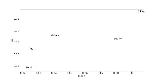
Let's first drop the incorrect definition of excess return, and plot excess mean versus standard deviation plots (to reiterate, as these are future the returns are automatically excess of the risk free rate). Note that means that everything on a straight line will have the same Sharpe Ratio.

Looks pretty good! And indeed if we look at the statistics including the Sharpe Ratios, we can see there is not that much difference between the SR, certainly nothing statistically significant:

        mean   std    sr
Ags     0.02  0.12  0.20
Bond    0.02  0.04  0.55
Equity  0.08  0.16  0.48
Metals  0.04  0.18  0.21
OilGas  0.09  0.28  0.34

Although we only have five data points, it does seem that there is a roughly positive relationship between excess mean over risk free and standard deviation.

Bringing in Beta

Having verified the original results after substituting the risk free rate for inflation, let's now bring in Beta. Under CAPM we'd expect that if we plotted excess mean against covariance rather than standard deviation, we'd again find a positive relationship. That should make assets with lower correlations look more attractive; that reminds me here's the correlation matrix:

        Ags  Bond  Equity  Metals  OilGas
Ags     1.00 -0.11    0.21    0.37    0.27
Bond   -0.11  1.00    0.09   -0.06   -0.14
Equity  0.21  0.09    1.00    0.26    0.12
Metals  0.37 -0.06    0.26    1.00    0.28
OilGas  0.27 -0.14    0.12    0.28    1.00

The problem of course is how to measure Beta, i.e. what is the 'market' that we are regressing our returns on. That's a hard enough problem when considering equities, but here we should really include every investable asset in the world, weighted by market cap back to 1983. I don't have those figures to hand!!

Instead I'm going to opt for another quick and dirty solution, namely to create a market index in the following proportions:

• Ags 10%
• Bonds 40%
• Equities 30%
• Metals 10%
• Oil and Gas 10%

This is based on some roughly true things; bonds and equities form most of the investable universe and there are more bonds issued than equities. And since most people are probably starting with a bonds/equities based portfolio, considering the diversification available versus something that is mostly that is probably a reasonable thing to do.

If you prefer you can do something else like risk parity (which would be about 50% bonds, with the other asset classes roughly splitting the rest), but it probably won't make that much difference. 

This market index has a standard deviation of 7.4% a year, and a mean of 4.8%; it's SR of 0.64 as you would expect is superior to it's constituents.

Let's have a look at the betas and alphas, also correlation with the market (corr), standard deviations and Sharpe Ratios:

          std   corr   beta     sr  alpha
Ags     0.119  0.471  0.765  0.199 -0.011
Bond    0.039  0.183  0.098  0.553  0.017
Equity  0.162  0.826  1.822  0.484 -0.008
Metals  0.176  0.566  1.353  0.215 -0.026
OilGas  0.277  0.541  2.027  0.338 -0.006

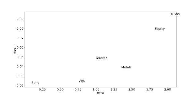
We can see that to an extent higher standard deviation also means higher beta, but not always; equities and metals have virtually the same standard deviation but equities have a higher beta because they are more correlated. There is also a weak relationship between alpha and SR.

Let's now redo the scatter plot but this time with Beta on the x-axis and adding the market portfolio:

The obvious outperformance of Bonds aside, this again does like a clear case of supporting the CAPM for the case of across asset classes; if anything it's clearer than before.

Intra market

Now let us address the point in the post which is mentioned but briefly; the fact that CAPM doesn't work within asset classes. This is not a new finding. Indeed there is the mysterious result of Beta making an excellent counter signal ('Betting against Beta' Pedersen and Frazzini JFE 2014) at least in individual equities. It seems that lower Beta stocks have excess Alpha compared to higher Beta stocks; one story that explains that is that if Beta is synomonous with standard deviation (which as discussed, it ain't exactly), then we'd need higher leverage to hold low Beta stocks and not everyone can or wants to leverage to the hilt.

This is perhaps a more interesting study to do, since we could potentially use any positive result here as a trading signal; buying instruments within an asset class that have low Beta (or low standard deviation), and shorting those that are high Beta. Once again we run up against the definition of 'the market' in each asset class, but I will stick with the simple equal weighted across time version I have been using so far.

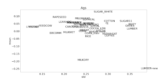
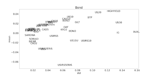
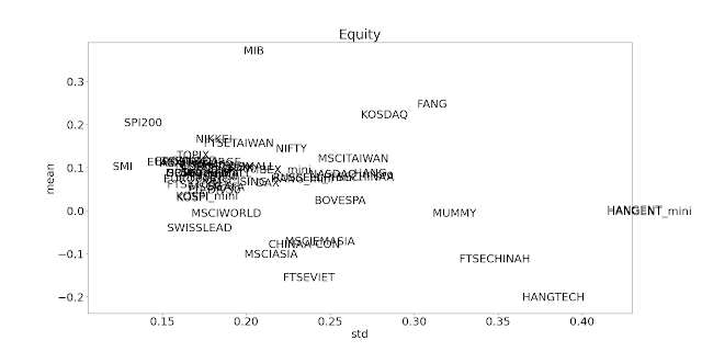
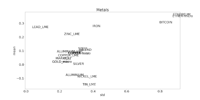
Here follows a blizzard (correct collective noun?) of plots. Firstly, here's excess mean against standard deviation (the original Sharpe Ratio plot):

A big caveat here is that different instruments may have wildly different data histories. With that said, there is mostly no evidence here of a similar Sharpe Ratio. The exception is bonds. There does seem to be a relationship between duration (which is highly correlated to standard deviation) and excess return; and we also see that High Yield which is riskier than most of the goverment bonds has a higher return. In other worse, the bastardised version of the CAPM using vol rather than Beta does work within one asset class, which is perhaps why the authors of the original post decided to treat bonds as several different asset classes :-)

Now let's do things 'properly' and look at excess mean versus Beta:

Interestingly the positive result in Bonds is slightly different here; it mostly holds true that we get higher excess return for more Beta with the exception of high yield bonds. These are negatively correlated to the rest of the universe, and as a result have negative Beta. My returns for the high yield bond future go back to 2000, so this isn't a fluke down to a limited number of returns. However for government bonds, again it seems that CAPM holds true.

For a giggle let's reproduce the plots from the 'Betting Against Beta' paper, and plot Alpha vs Beta. CAPM predicts a horizontal line, whilst the original paper found a downward sloping line.

With the possible exception of oil and gas, there isn't much to write home about here. It doesn't look like CAPM or Betting against Beta is particularly compelling within asset classes that contain futures. 

(Note that in any case this isn't a proper test of Betting against Beta as a trading signal, since everything is in sample and not time varying)

Summary

Sloppy execution aside, the key findings of the original paper are correct; CAPM doesn't really work within asset classes, unless you lump all bonds into a single asset class in which case it works just fine, but it does work across asset classes. 

Percentage or price differences when estimating standard deviation - that is the question

In a lot of my work, including my new book, I use two different ways of measuring standard deviation. The first method, which most people are familiar with, is to use some series of recent percentage returns. Given a series of prices p_t you might imagine the calculation would be something like this:

Sigma_% = f([p_t - p_t-1]/p_t-1, [p_t-1 - p_t-2]/pt-2, ....)

NOTE: I am not concerned with the form that function f takes in this post, but for the sake of argument let's see it's a simple moving average standard deviation. So we would take the last N of these terms, subtract the rolling mean from them, square them, take the average, and then take the square root.

For futures trading we have two options for p_t: the 'current' price of the contract, and the back adjusted price. These will only be the same in the days since the last roll. In fact, because the back adjusted price can go to zero or become negative, I strongly advocate using the 'current' price as the denominator in the above equation, and the changein back adjusted price as the numerator. If we used the change in current price, we'd see a pop upwards in volatility every time there was a futures roll. So if p*_t is the current price of a contract, then:

Sigma_% = f([p_t - p_t-1]/p*_t-1, [p_t-1 - p_t-2]/p*t-2, ....)

The alternative method, is to use some series of price differences:

Sigma_d = f([p_t - p_t-1], [p_t-1 - p_t-2], ....)

Here these are all 

If I wanted to convert this standard deviation into terms comparable with the % standard deviation, then I would divide this by the current price (*not* the backadjusted price):

Sigma_d% = Sigma_d / p*_t

Now, clearly these are not going to give exactly the same answer, except in the tedious case where there has been no volatility (and perhaps a few, other, odd corner cases). This is illustrated nicely by the following little figure-ette (figure-ine? figure-let? figure-ling?):

import pandas as pd
perc =(px.diff()/pxc.shift(1)).rolling(30, min_periods=3).std()
diff = (px.diff()).rolling(30, min_periods=3).std().ffill()/pxc.ffill()
both = pd.concat([perc,diff], axis=1)
both.columns = ['%', 'diff']

The two series are tracking pretty closely, except in the extreme vol of late 2008, and even they aren't that different. 

Here is another one:

That's WTi crude oil during COVID; and there is quite a big difference there. Incidentally, the difference could have been far worse. I was trading the December 2020 contract at the time... the front contract in this period (May 2020) went below zero for several days.

Now most people are more familiar with % standard deviations, which is why I have used it so much, but what you may not realise is that the price difference standard deviation is far more important.

How come? Well consider the basic position sizing equation that I have used throughout my work:

N = Capital × τ ÷ (Multiplier × Price × FX rate × σ_% )

(This is the version in my latest book, but very similar versions appear in my first and third books). Ignoring most things we get:

N = X ÷ (Price × σ_%)

So the number of contracts held is proportional to one divided by the price multiplied by the percentage standard deviation estimate. The price shown is, if you've been paying attention, the current price not the back adjusted one. But remember:

Sigma_d% = Sigma_d / p*_t

Hence the position is actually proportional to the standard deviation in price difference terms. We can eithier estimate this directly, or as the equation suggests recover it from the standard deviation in percentage terms, which we then multiply by the current futures price.

As the graphs above suggest, in the majority of cases it won't make much difference which of these methods you choose. But for the corner case of prices close to zero, it will be more robust to use price differences. In conclusion: I recommend using price differences to estimate the standard deviation.

Finally, there are also times when it still makes sense to use % returns. For example, when estimating risk it's more natural to do this using percentages (I do this when getting a covariance matrix for my exogenous risk overlay and dynamic optimisation). When percentage standard deviation is required I usually divide my price difference estimate by the absolute value of the current futures price. That will handle prices close to zero and negative prices, but it will result in temporarily very high % standard deviations. This is mostly unavoidable, but at least the problem is confined to a small part of the strategy, and the most likely outcome is that we won't take positions in these markets (probably not a bad thing!).

Footnote: Shout out to the diff(log price) people. How did those negative prices work out for you guys?