Happy new year.
I didn't post very much in 2022, because I was in the process of writing a new book (out in April!). Save a few loose ends, my work on that project is pretty much done. Now I have some research topics I will be looking at this year, with the intention of returning to something like a monthly posting cycle.
To be clear this is *not* a new years resolution, and therefore is *not* legally or morally binding.
The first of these research projects relates to expensive (high cost) trading strategies. Now I deal with these strategies in a fairly disdainful way, since I'm conservative when it comes to trading fast and I prefer to avoid throwing away too much return on (certain) costs in the pursuit of (uncertain) returns.
Put simply: I don't trade anything that is too quick. To be more precise, I do not allocate risk capital to trading rules where turnover * cost per trade > 'speed limit'. The effect of this is that instruments that are cheaper to trade get an allocation to expensive trading rules that have a high turnover; but most don't. And there are a whole series of potential trading rules which are far too rich for all but the very cheapest instruments that I trade.
My plan is to do a series of posts that explore in more depth whether this is the correct approach, and whether there is actually some room for faster trading strategies in my quiver. Broadly speaking, it might be that eithier:
- The layers of buffering and optimisation in my system mean it is possible to add faster strategies without worrying about the costs they incur.
- Or there could be some other way of smuggling in faster trading, perhaps via an additional execution layer that optimises the execution of orders coming from the (slow) core strategy.
Part of the motivation for this is that in my new book I introduce some relatively quick trading strategies which are viable with most instruments, but which require a different execution architecture from my current system (a portfolio that is dynamically optimised daily, allowing me to include over 100 instruments despite a relatively modest capital base). Thus the quicker strategies are not worth trading with my retail sized trading account; since to do so would result in a severe loss of instrument diversification which would more than negate any advantages. I'll allude to these specific strategies further at some point in the series, when I determine if there are other ways to sneak them into the system.
For this first post I'm going to explore the relationship between instrument cost and momentum performance. Mostly this will be an exercise in determining whether my current approach to fitting instrument and forecast weights is correct, or if I am missing something. But it will also allow me to judge whether it is worth trying to 'smuggle in' faster momentum trading rules that are too pricey for most instruments to actually trade.
The full series of posts:
- This is the first post
- The second post discusses whether fast trading rules can be 'smuggled in' to my existing system
Note 1: There is some low quality python code here, for those that use my open source package pysystemtrade. And for those who haven't yet pre-ordered the book, you may be interested to know that this post effectively fleshes out some more work I present in chapter nine around momentum speed.
Note 2: The title comes from this song, but please don't draw any implications from it. It's not my favourite Geri Halliwell song (that's 'Look at Me'), and Geri isn't even my favourite Spice Girl (that's Emma), and the Spice Girls are certainly not my favourite band (they aren't even in my top 500).
The theories
There are two dogs in this fight.
Well metaphorical dogs, I don't believe in dog fighting. Don't cancel me! But the fight is very real and not metaphorical at all.
I'm interested in how much truth there is in the following two hypothesis:
- We have a prior belief that the expected pre-cost performance for a given trading rule is the same regardless of underlying instrument cost.
- "No free lunch": expected pre-cost performance is higher for instruments that cost more to trade, but costs exactly offset this effet. Therefore expected post-cost performance for a given trading rule will be identical regardless of instrument cost.
I use expectations here because in reality, as we shall see, there is huge variation in performance over instruments but quite a lot of that isn't statistically significant.
What implications do these hypothesis have? If the first is true, then we shouldn't bother trading expensive instruments (or at least radically downweight them, since there will be diversification benefits). They are just expensive ways of getting the same pre-cost performance. But if the second statement is true then an expensive instrument is just as good as a cheaper one.
Note that my current dynamic optimisation allows me to side step this issue; I generate signals for instruments regardless of their costs and I don't set instrument weights according to costs, but then I use a cost penalty optimisation which makes it unlikely I will actually trade expensive instruments to implement my view. Of course there are some instruments I don't trade at all, as their costs are just far too high.
Moving on, the above two statements have the following counterparts:
- We have a prior belief that the expected pre-cost performance across trading rules for a given instrument is constant.
- Expected post-cost performance across trading rules for a given instrument will be identical.
What implications do these theories have for deciding how fast to trade a given instrument, and how much forecast weight to give to a given speed of momentum? If pre-cost SR is equal, we should give a higher weight to slower trading rules; particularly if an instrument is expensive to trade. If post-cost SR is equal, then we should probably give everything equal weights.
Note that I currently don't do eithier of these things: I completely delete rules that are too quick beyond some (relatively arbitrary) boundary, then set the other weights to be equal. In some ways this is a compromise between these two extremes approaches.
A brief footnote:
You may ask why I am looking into this now? Well, I was pointed to this podcast by an ex-colleague, in which another ex-colleague of mine makes a rather interesting claim:
"if you see a market that is more commoditised [lower costs] you tend to see faster momentum disappear."
Incidentally it's worth listening to the entire podcast, which as you'd expect from a former team member of yours truely is excellent in every way.
Definitely interesting! This would be in line with the 'no free lunch' theory. If fast momentum is only profitable before costs for instruments that cost a lot to trade, then it won't be possible to exploit it. And the implication of this is that I am doing exactly the wrong thing: if an instrument is cheap enough to trade faster momentum, I shouldn't just unthinkingly let it. Conversely if an instrument is expensive, it might be worth considering faster momentum if we can work out some way of avoiding those high costs.
It's also worth saying that there are already some stylised facts that support this theory. Principally, faster momentum signals stopped working particularly in equity markets in the 1990s; and equity markets became the cheapest instruments to trade in the same period.
Incidentally, I explore the change in momentum profitability over time more in the new book.
The setup
I started with my current set of 206 instruments, and removed duplicates (eg mini S&P 500, for which the results would be the same as micro), and those with less than one year of history (for reasons that will become clearer later, but basically this is to ensure my results are robust). This left me with 160 instruments - still a decent sample.
I then set up my usual six exponentially weighted moving average crossover (EWMAC) trading rules, all of the form N,4N so EWMAC2 denotes a 2 day span minus an 8 day span: EWMAC2, EWMAC4, EWMAC8, EWMAC16, EWMAC32, EWMAC64.
I'm going to use Sharpe ratio as my quick and dirty measure of performance, and measure trading costs per instruments as the cost per trade in SR units. However because the range of SR trading costs is very large, covering several orders of magnitude (from 0.0003 for NASDAQ to over 90 for the rather obscure Euribor contract I have in my database), I will use log(costs) as my fitting variable and for plotting purposes.
Before proceeding, there is an effect we have to bear in mind, which is the different lengths of data involved. Some instruments in this dataset have 40+years of data, others just one. But in a straight median or mean over instrument SR they will get the same weighting. We need to check that there is no bias; for example because equities generally have less data and are also the cheapest:

Here the y-axis shows the SR cost per trade (log axis) and the x-axis shows the number of days of data.
There doesn't seem to be a clear bias, eg more recent instruments especially cheap, so it's probably safe to ignore the data length issue.
Gross SR performance by trading rule versus costs


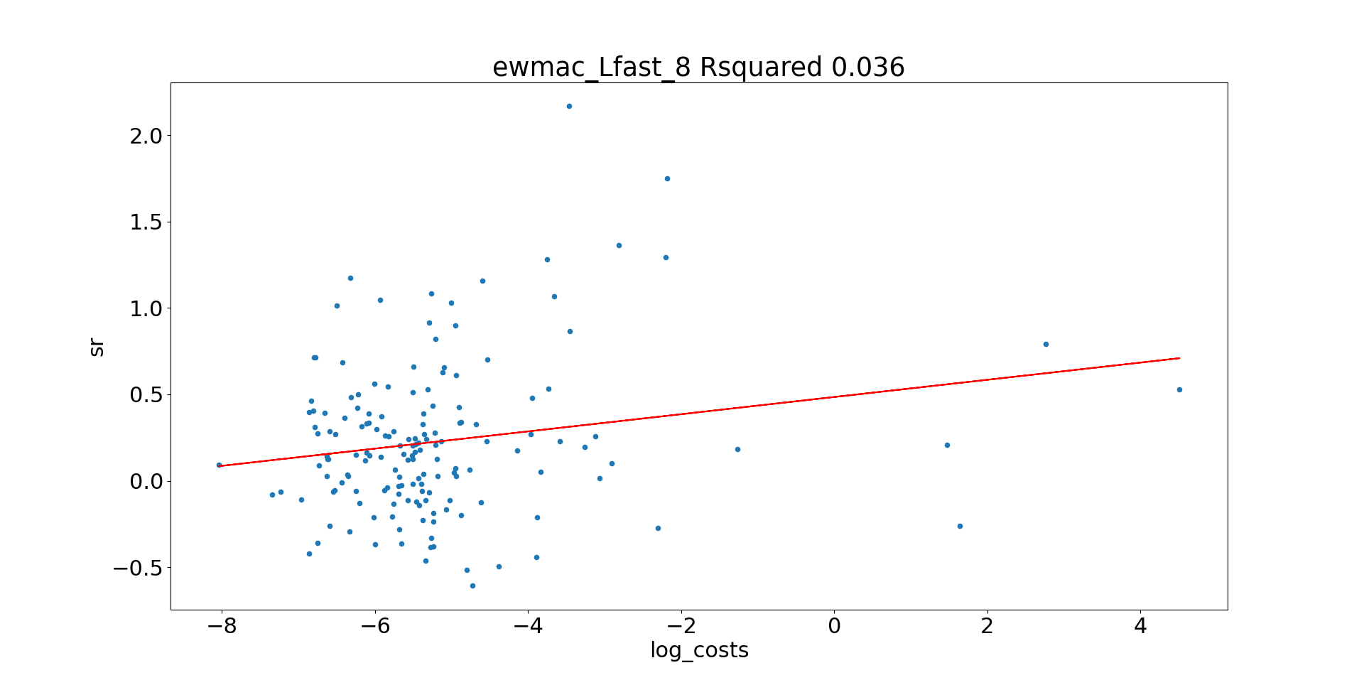


Net SR performance by trading rule versus costs

Technically I should allow for the effect of rolls on turnover but in for simplicity I ignore those when drawing the red line, since roll frequency is different for each instrument. They will only have an effect for very expensive instruments at very slow speeds.


Optimal trading speed
Let's return to the second set of statements we want to test:
- We have a prior belief that the expected pre-cost performance across trading rules for a given instrument is constant.
- Expected post-cost performance across trading rules for a given instrument will be identical.
- Identical regardless of instrument costs
- Faster for more expensive instruments
- Slower for more expensive instruments
- Identical regardless of instrument costs
speed_as_list = np.array([1,2,3,4,5,6])
def optimal_trading_rule_for_instrument(instrument_code, curve_type="gross"):
    sr_by_rule = pd.Series([
        sr_for_rule_type_instrument(rule_name, instrument_code, curve_type=curve_type)
        for rule_name in list_of_rules])

    sr_by_rule[sr_by_rule<0] = 0
    if sr_by_rule.sum()==0:
        return 7.0

    sr_by_rule_as_weight = sr_by_rule / sr_by_rule.sum()
    weight_by_speed = sr_by_rule_as_weight * speed_as_list
    optimal_speed = weight_by_speed.sum()

    return optimal_speed
Optimal trading speed with gross SR

Well this looks pretty flat. The optimal trading speed is roughly 3.5 (somewhere between EWMAC8 and EWMAC16) for very cheap instruments, and perhaps 3 for very expensive ones. But it's noisy as anything. It's probably safe to assume that there is no clear relationship between optimal speed and instrument costs, if we only use gross returns.
Optimal trading speed with net SR
Now let's do the same thing, but this time we find the optimal speed using net rather than gross returns.

There are a lot more '7' here, as you'd expect, especially for high cost instruments (which all have negative SR after costs for all momentum), but there are also quite a few lower cost instruments with the same problem. This is just luck - we know that SR by trading rule is noisy, so by bad luck we'd have a few instruments which have negative SR for all our trading rules.
As we did before, let's ignore the instruments above the red line, and run a regression on what's left over:


To trade EWMAC64 and nothing else, I'd require an instrument SR cost of less than 0.021 (again assuming quarterly rolls; it would be higher for monthly rolls), or -3.8 in log space. With costs higher than that I couldn't trade anything at all.
Note that is to the left of the red line, since the red line ignores the effect of rolling on turnover.
Just EWMAC64 is a speed number of 6, and the regression suggests a speed number of 5.9 with -3.8 log costs. That is a pretty good match.
Happy New Year, Rob!
ReplyDeleteHappy New Year to all of your readers!