This is a blog post which has been coming for a while. It relates to a lot of themes I've discussed before, and a recurring conversation I've had with a few people.
As most regular readers will know, I run my trading strategy to hit a particular risk target. That risk target is expressed as an annual standard deviation of percentage returns, and happens to be 25%. But those details aren't that important here. What is important is that it is a long run average risk target. Over the long run the expected risk in my backtest should be (pretty close to) 25% on average. If I can do a reasonable job of forecasting risk (and I usually can), then the actual ex-post standard deviation of returns in my backtest should also be 25% on average.
The important word here is on average. On a given day, my actual expected risk may be quite different from 25%. As I've discussed before, this is for two reasons. The first is something that I'm quite keen on: forecasting. A higher forecast means we have higher conviction in our trades, and thus our expected risk should be higher. The second thing is more of an annoyance: the relative correlation factor. It reflects the fact that my system is calibrated to size positions based on average historic correlations between market returns and positions. But on any given day these could be quite different, resulting in radically different expected risk.
There is no law saying you have to construct a trading strategy in this way. You could, for example, adjust your positions so that your expected risk is constant. Indeed this is common amongst long/short equity neutral funds which have historically tended to follow the classic Fama/French style factor model. Typically they go long the top quintile of their stock universe and go short the bottom quintile*. There is only a coarse link between forecast and position size here; everything is eithier in the portfolio as a long or short, or not in the portfolio at all (more formally, the relationship between forecast and position size is a thresholded binary mapping). The expected risk of this portfolio will depend only on todays covariance matrix. It makes perfect sense then to adjust the sizes of the resulting positions to target a fixed risk level.
* I've clearly simplified things a lot here; most funds will adjust positions to hit a zero net Beta and may also neutralise sector and/or certain factor exposure.
Could we then apply such an approach to a system like mine that does use forecasts? Clearly, the main disadvantage of this approach is that you lose any information provided by the forecasts. In a period when forecasts were generally low, we'd gear up our positions to hit the target risk, and the converse would be true when forecasts were low. But that might not matter: if our portfolio is diversified enough then the range of dispersion in aggregate forecasts might not be that big. And another benefit could plausibly be an improvement in the characteristics of the portfolio. After all, vol targeting makes sense on a position level, so why not a portfolio level?
In this post I'll explore the idea of fixing ex-ante portfolio risk, and also propose a possible 'best of both worlds' compromise to this binary argument.
As I've already noted this post links to several previous posts:
- It's part three of a four(?) part series on forecasting, which started with this post. In that post I showed that forecasting mostly 'works' for individual instruments, with the caveat that there was some non linearity in the response of risk adjusted expected returns to forecasts (part of which can be explained by biased vol forecasting).
- In this older post I looked at volatility targeting on a position sizing level. Not quite the same, but interesting nonetheless. I found that vol targeting improved Sharpe Ratio and kurtosis, but reduced positive skew. I'll be looking at higher moment effects in this post as well.
- I'll draw heavily on this post I did on risk management to explain how forecasts influence expected risk, and where I also showed to calculate portfolio risk in pysystemtrade.
Why does expected risk vary?
This section is a direct copy from this post I did on risk management, so feel free to skip it if you remember something I wrote 5 whole months ago (I don't!).
The expected risk of my portfolio todaywill be wSw', where w are the current weights (basically position as % of capital) and S is my current estimate of the covariance matrix composed of instrument standard deviations and the correlation between instrument returns.The position measured as a percentage of capital is a product of a lot of different numbers, but it simplifies to this:
position as % of capital = (instrument forecast / average instrument forecast)* (target risk / instrument risk) * instrument weight * IDM
Where the IDM (Instrument Diversification Multiplier) is the factor applied to positions to account for the correlation between trading subsystems (i.e. the trading strategies we run for each instrument and the returns they product, not the underlying instrument returns we use for S).
In a very handwaving way, it can be shown that the current expected portfolio risk will then be equal to:
Expected risk = target risk * (relative forecast strength) * (relative correlation factor)
Relative forecast strength is a measure of how strong aggregate forecasts are relative to the average; it is equal to the absolute forecasts for each instrument, weighted by instrument weight and divided by the average forecast (set to 10 in pysystemtrade).
All other things being equal, if your forecasts are all +20, and the average is +10, then your expected portfolio risk would be twice the average risk, or roughly twice the target risk (50% in the example I've been using).
This assumes that we want risk to vary according to aggregate forecast strength. Otherwise we'd have exactly the same risk on even if our forecasts were all +0.001, as if they were +20 (the maximum allowed under forecast capping). I'll check this assumption later in the post.
The relative correlation factor (RCF) is a bit more complicated. It is equal to the ratio between the IDM (which accounts for the average correlation across subsystem returns), and the IDM that would be appropriate today given the current set of positions and current correlation between instrument returns.
So for example, if you normally trade two subsystems (say US 10 year and S&P 500) with corelation between subsystems of zero then your IDM will be equal to square root of 2: 1.414
Now imagine that for some reason your system has a long average sized position in US 10 years, and a short average sized position in S&P 500 futures, and also that the correlation between these two instruments is -1. A quick calculation shows that the expected risk here will be 2.82 times the average. If the correlation was zero, then the expected risk would be twice the average; and if the correlation was +1 then the expected risk would be zero. The relevant RCF would be 2.82/1.41, 2/1.41, and zero.
Clearly the RCF can vary quite a lot depending on what the current positions are, and the current correlation matrix. You might argue that positions and correlations of this kind are unlikely given the average correlation between subsystems is zero. They are unlikely, but they aren't impossible. In particular, correlations do vary especially in the kind of market conditions we saw in March 2020.
The RCF is more of an annoyance in terms of expected risk; we wouldn't neccessarily want our risk to be a lot higher just because the positions we happen to have on are especially toxic given what todays correlations just happen to be.
... and if you've skipped, the rest of this post is original material.
Fixing portfolio risk
So we have a problem: the RCF means that our expected risk will move around quite a bit, regardless of our forecasts. And we have a possible solution, which is to fix the ex-ante expected portfolio risk.
It's trivial to do this. Firstly we measure the expected risk of our portoflio Sp using the bolierplate portfolio risk calculation which is wSw', where w are the weights (basically position as % of capital) and S is the covariance matrix composed of instrument standard deviations and the correlation between instrument returns (different from that used for IDM).
We then calculate a risk adjustment factor, f = St / Sp where St is our risk target. Finally we multiply all our positions by f.
And this solution itself creates another problem! As I said above:
Expected risk = target risk * (relative forecast strength) * (relative correlation factor)
This means that f will be equal to:
f = 1/ [(relative forecast strength) * (relative correlation factor)]
Our adjusted expected risk, after applying f, will be:
Expected risk = target risk
We've dealt with the dirty bathwater which the RCF is floating in, but we've also thrown out the baby that is the relative forecast strength. Is this a bad idea, or not?
How variable are forecasts at an aggregate level?
f = 1/ relative correlation factor
def forecast__strength_for_system(system):
    list_of_instruments = system.get_instrument_list()
    forecasts = [system.combForecast.get_combined_forecast(instrument_code)
              for instrument_code in
                list_of_instruments]
    forecasts = pd.concat(forecasts, axis=1)
    forecasts.columns = list_of_instruments
    forecasts = forecasts / system.config.average_absolute_forecast
    instrument_weights = system.portfolio.get_instrument_weights()

    weighted_forecast = instrument_weights.ffill() * forecasts.abs().ffill()
    forecast_strength = weighted_forecast.sum(axis=1)

    return forecast_strength
 |
| Aggregate absolute forecast weighted by instrument weights |
Do forecasts have forecasting power at an aggregate level?
def get_future_portfolio_return(Ndays):
    acc_curve = system.accounts.portfolio()
    acc_curve_sum = acc_curve.cumsum()
    period_returns = acc_curve_sum - acc_curve_sum.shift(Ndays)

    # We apply a single risk adjustment
stdev = acc_curve.std()
scaled_returns_vol = stdev * (Ndays**.5)
normalised_return = period_returns / scaled_returns_vol
future_normalised_return = normalised_return.shift(-Ndays)
return future_normalised_return
Ndays = 30
future_norm_return = get_future_portfolio_return(Ndays)
agg_forecast = forecast_strength_for_system(system)
pd_result = pd.DataFrame(dict(x=agg_forecast, y = future_norm_return))
plot_results_for_bin_size(6, pd_result, centre_on_mean=True) |
| Y-axis: risk adjusted ex-post portfolio return. X-axis: |
What effect does imposing a fixed risk target have on portfolio returns?
acc_curve = system.accounts.portfolio()

risk_series = get_expected_risk_for_system(system)
risk_series = risk_series.ffill()
# zero risk is bad because infinity
risk_series[risk_series==0]=np.nan
risk_vs_target = 100*risk_series / system.config.percentage_vol_target
risk_multiplier = 1/risk_vs_target# let's not get carried away here guys
risk_multiplier[risk_multiplier>3.0] = 3.0
acc_curve_with_risk_multiplier = acc_curve * risk_multiplier
acc_curve.cumsum().plot()acc_curve_with_risk_multiplier.cumsum().plot() |
| Red line: Account curve without fixed risk targeting. Blue curve: Account curve with fixed risk targeting |
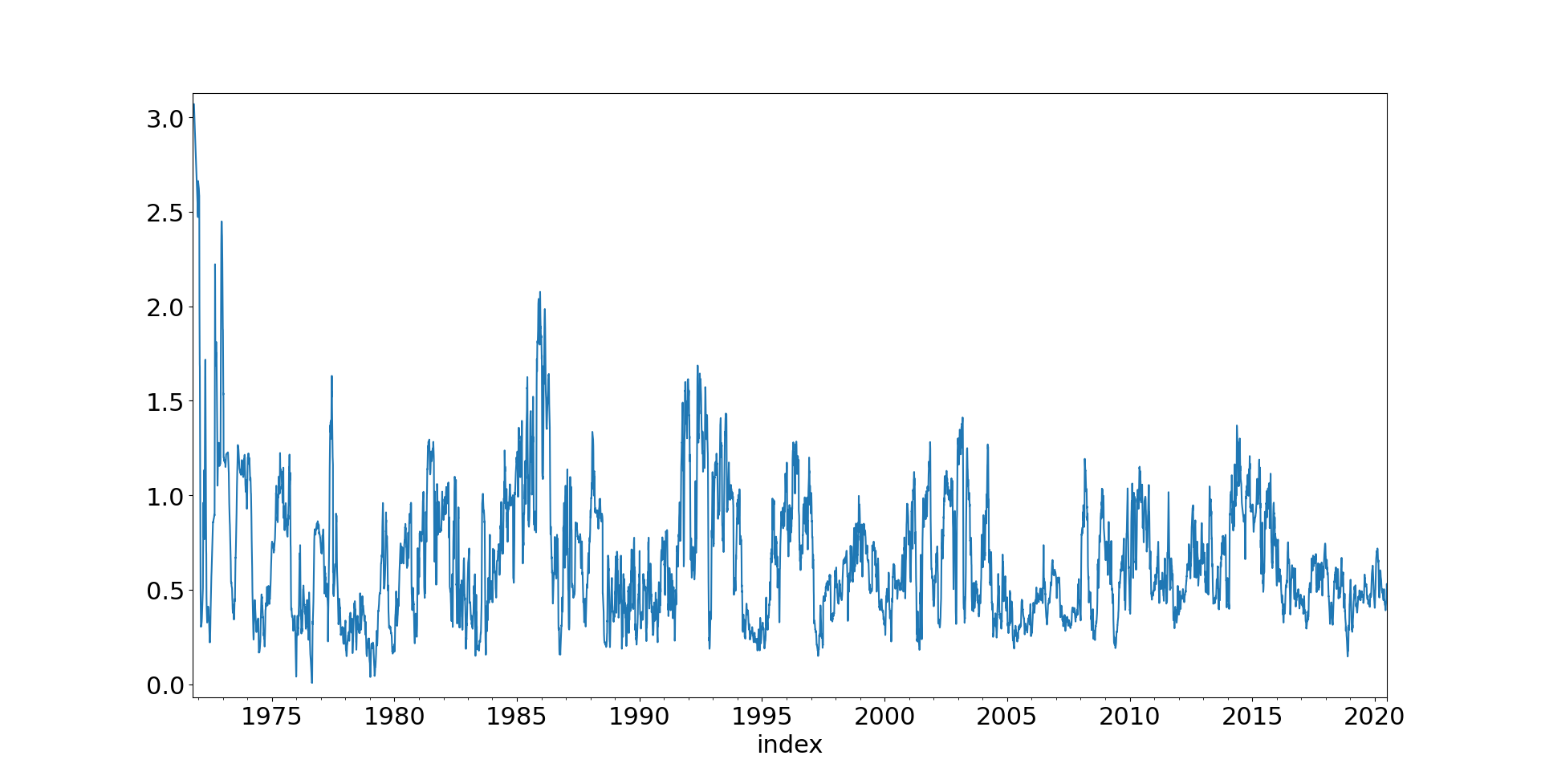
 |
| Y-axis: Rolling 6 month realised daily standard deviation of returns. Blue line: Original System. Orange line: Fixed risk target |
Can we use forecasts but account for changes in correlation and positions?
Let's return again to this equation:
Expected risk = target risk * (relative forecast strength) * (relative correlation factor)What we really want is something that does something like this:Expected risk = target risk * (relative forecast strength)
We've tried targeting a fixed risk, which means multiplying all our positions by f: f= St / Sp (where St is our risk target and Sp is our portfolio risk)f = 1/ [(relative forecast strength) * (relative correlation factor)]
And that didn't go well. But what if we multiplied our positions by f*, which is f multiplied by the relative forecast strength:
f= (relative forecast strength)*St / Sp f* = (relative forecast strength)/ [(relative forecast strength) * (relative correlation factor)] = 1 / (relative correlation factor)]Now we're cooking with some kind of petroleum vapour! f* only corrects for the relative correlation factor, leaving forecast strength to be unaffected.What does this look like in code:risk_multiplier_forecasts = (agg_forecast/agg_forecast.mean())*risk_multiplier
acc_curve_with_forecast_risk_multiplier = acc_curve * risk_multiplier_forecasts
Since the aggregate forecast measure isn't guaranteed to have a mean of 1, we account for this. |
| Red line: Account curve without fixed risk targeting. Blue curve: Account curve with fixed risk targeting, accounting for forecast magnitude |
Rob, I have read this post and the chapters/sections on Volatility Targeting in AFTS and ST. I would like to apply these principles to a non-correlated portfolio of 6 cross margined SMAs managed by CTA hedge fund managers. I have 62 months of common historical monthly data for each manager's after fee performance. From the covariance matrix, I derive a 7.7% annual expected CAGR on volatility of 6.4% on notional. Looking at drawdown and margin/equity individual histories and adding some cushion I am comfortable with a leverage ratio in the cross margined SMA of 2.38%. I intend to apply your principles to this portfolio and set a volatility limit of 25% on trading capital annually. My question is how much daily or monthly divergence from the annual 25% vol limit would you accept before acting to limit the trading levels of the individual managers?
ReplyDeleteI assume for simplicity all the managers are targeting the same vol (which if they are all CTA's I would imagine is about 10% given you end up with 6.4% vol on the portfolio). One starting point is this post https://qoppac.blogspot.com/2022/02/exogenous-risk-overlay-take-two.html where you can see that 'normal risk' for my system varies between 0.5 and 1.5 times the risk target. That is expected risk, realised risk will vary a bit more, and it will also vary more for a CTA that is a purer trend follower with less diversification. 62 months isn't really enough to give you an indication of whether say a 3 times risk is typical for a given manager.
DeleteHi rob, I've been developing my own trading system based off your framework in systematic trading and I've been experimenting with dynamic calculation of forecast scalars using a 252 day EMA of absolue forecasts produced by each trading rule to estimate a historical absolute value of the forecast. However I've found that my performance suffers in markets that have been rangebound for long periods of time because the estimation of the average absolute forecast seems to be deflated (compared to an average across many assets and longer periods of time) and thus pushing up the value of the forecast scalars which makes forecasts in low trend environments to be inflated. Would increasing my lookback window help or should I just use all data across all assets? I find that having this dynamic scalar estimation makes it much easier for me to develop new trading rules and maintain a target portfolio volatility because I don't need to backtest across many assets.
ReplyDeleteI expressly say not to do this and you have independently discovered why. It might just about work for a very fast signal but for a very slow signal you will get scalars that are biased by the current market regime. I always use a lookback of infinity, averaging across all markets, to estimate forecast scalars. For some forecasts you can use random data to estimate what the scalar should be.
DeleteThank you for your reply Rob. Do you think that a dynamic Forecast Diversification Multiplier (FDM) that is calculated based off of a rolling window of correlations between trading rule forecasts or returns would work? If so, will there be any significant differences between using forecasts and returns for the calculation?
DeleteAgain, why you use a rolling window? There is no reason to expect correlations of forecasts to change over time so you are just introducing noise. It shouldn't make any significant difference if you use returns or forecasts it's just easier and simpler to use forecasts.
Delete