This is a blog post about forecasting vol. This is important, since as sensible traders we make forecasts about risk adjusted returns (as in my previous post), which are joint forecasts of return and volatility. We also use forecasted vol to size positions. A better vol forecast should mean we end up with a trading strategy that has a nicer return profile, and who knows maybe make some more money.
Mean reverting vol, and it's effect on forecast accuracy
In my previous post I looked at the non linear response of risk adjusted returns to forecast values. There were many plots like this one:
 |
| Forecast and subsequent risk adjusted return for ewmac16_64 trading rule for Gold. Mean risk adjusted return for 12 buckets, conditioned on sign and distributional points of forecast. |
What we expect is that as a forecast gets stronger, the risk adjusted return also gets stronger. This plot (with forecast on the x-axis, and subsequent risk adjusted return over the holding period of the trading rule) should then show a linear response. But we don't see that; instead we see this 'reversion to the wings' pattern: for strong forecasts (of eithier sign) the response is actually weaker than we'd expect.
Although this is a particularly striking plot, there are is a similar effect if I pool results across all instruments. You may recall from the post that the effect is non existent for fast momentum, but relatively high in slower momentum (and also, though I didn't dig into it, carry).
This pattern is annoying, although one quick fix is to use a capped forecast, which essentially collapses the problem in the tails and makes things not quite as bad. Still, it's annoying: the previous post was about non binary forecasts being better than binary, and this effect narrows the gap somewhat by reducing the performance of non binary forecasting when forecasts get a bit heavy.
Here is a key paragraph from the previous post:
"This is a pretty well known effect in trend following, and there are a few different explanations. One is that trends tend to get exhausted after a while, so a very strong trend is due a reversal. Another is that high forecasts are usually caused by very low volatility (since forecasts are in risk adjusted space, low vol = high forecast), and very low vol has a tendency to mean revert at the same time as markets sharply change direction."
In this post I'm going to focus on the second part of this sentence. Let me explain a bit more clearly what I mean.
We know that forecast = expected return / expected volatility. I use a very simple measure of expected volatility, which is equal to historic volatility over the last month or so (actually exponentially weighted, but with an equivalent half life), so we actually have: forecast = expected return / recent volatility. There are clearly two reasons why forecasts could be high: if expected return is relatively high, or if recent volatility is particularly low.
Now the risk adjusted ex post return is similarly defined as return = actual return / actual volatility. Thus if actual volatility is much higher than expected volatility (hence mean reverting), even if we get the expected return spot on, we'll see lower ex post risk adjusted returns when forecasts are large because vol is lower.
Mean reverting vol, and it's effect on forecast accuracy
It's very easy to see if this is what is happening. We can do a similar plot as before, except now we're going to plot forecast on the x-axis, and the ratio of actual versus expected vol on the y-axis. Effectively then this is a measure of how good we are at forecasting vol, conditional on forecast strength.
Mostly this uses the same code as last time, but I replace get_forecast_and_normalised_return() with this:
def get_forecast_and_normalised_vol(instrument, rule): # uncomment depending on which forecast to use
#forecast = system.forecastScaleCap.get_capped_forecast(instrument, rule)
forecast = system.forecastScaleCap.get_scaled_forecast(instrument, rule)
# holding period
Ndays = int(np.ceil(get_avg_holding_period_for_rule(forecast)))
forecast_vol = system.rawdata.get_daily_percentage_volatility(instrument)
future_vol = get_future_vol(instrument, Ndays)
ratio_vol = future_vol / forecast_vol
ratio_vol = ratio_vol.ffill()
pd_result = pd.concat([forecast, ratio_vol], axis=1)
pd_result.columns = ['forecast', 'ratio_vol']
pd_result = pd_result[:-Ndays]
return pd_result
def get_future_vol(instrument_code, Ndays): # Unlike the forecast vol (recent current vol) this isn't EWMA
returns = system.rawdata.get_percentage_returns(instrument_code)
stdev = returns.rolling(Ndays, min_periods = 3).std()
future_stdev = stdev.shift(-Ndays)
return future_stdev
I'm going to do these plots as before with 'bins=6' (to show the granularity of the response), over all my various trading rules, with data summed across all instruments.
Referring back again to the previous post we know that the 'reversion in the wings' for forecast responses is non existent for faster momentum, but for slow momentum we know the reversion is pretty fat, so let's plot the vol forecasting ratio and see what it looks like for ewmac_64_256:
 |
| Vol forecast accuracy conditioned on risk adjusted return forecast values, without capping. Rule 'ewmac64_256', data summed across all instruments. X-axis: forecast value, Y-axis: actual volatility over holding period divided by expected volatility when forecast was made |
If we were as good as forecasting vol, irrespective of forecast, this would be a flat line intercepting the y-axis at y=1 (assuming our vol forecasts were generally unbiased). But we don't see that! When forecasts are large, actual vol turns out to be relatively high compared to expected vol (ratio>1). When forecasts are small, actual vol is a little lower than expected. This is exactly what we'd expect if vol was mean reverting.
 |
| Vol forecast accuracy conditioned on risk adjusted return forecast values, with capping. Rule 'ewmac64_256', data summed across all instruments. X-axis: forecast value, Y-axis: actual volatility over holding period divided by expected volatility when forecast was made |
Is this a conditional effect, or are we just bad at vol forecasting?
There are a couple of explanations for what we've seen. One is that vol is indeed mean reverting, regardless of risk adjusted return forecast value. The other is that we get uniquely bad at forecasting vol when forecasts are really big.
It's important to distinguish between these two effects, because our fix will be different. If the effect is related to forecast size, then we should probably fit some kind of smoothed line through the vol ratio plots, and use that to adjust our vol forecasts (and hence our risk adjusted return forecast), conditional on the current forecast level.
If however the effect is entirely down to vol mean reverting, then we should probably try and do a better job of vol forecasting, independent of forecasting risk adjusted returns. And indeed, doing a better job of vol forecast seems like a noble goal in itself.
Here's some code:
def get_forecast_vol_and_future_vol(instrument, Ndays):
    vol = system.rawdata.get_daily_percentage_volatility(instrument)
    future_vol = get_future_vol(instrument, Ndays)

    ratio_vol = future_vol / vol
    ratio_vol = ratio_vol.ffill()

    slow_vol = vol.ewm(2500).mean()

    adj_vol = (vol / slow_vol)-1.0

    pd_result = pd.concat([adj_vol, ratio_vol], axis=1)
    pd_result.columns = ['historic_vol', 'ratio_vol']

    pd_result = pd_result[:-Ndays]

    return pd_result
'ratio_vol' we have seen before, but the conditioning variable now is 'adj_vol' which is the ratio of current (ex-ante) volatility and a very slow moving average of that, minus 1. So 'adj_vol' is equal to 0, then current volatility is at a similar level to what we have seen over the last 10 years or so. If it's strongly negative, then current volatility is low relative to recent history, and if it's strongly positive then vol is relatively high.
Let's do our usual plot, using a holding period ('Ndays') of 40 (roughly the same as ewmac64_256), but this time we plot the vol forecast ratio (ex-post vol / ex-ante vol) on the y-axis conditioned on the adjusted vol level (ex-ante vol / historic vol) on the x-axis:
 |
| Vol forecast accuracy conditioned on current level of volatility, data summed across all instruments. X-axis: (actual volatility / 10 year average volatility)-1, Y-axis: actual volatility over holding period divided by expected volatility when forecast was made |
If our vol forecasts were unbiased regardless of whether vol is high or low, we'd expect to see a flat horizontal line here, intercepting the y-axis at 1.0. Instead however, the vol ratio is above 1 when vol is currently low, and below 1 when vol is currently high. In other words, when vol is low we'll tend to understimate what it will be in the future (vol ratio>1: ex-post vol>ex-ante vol), and when vol is high we will over estimate it.
We have vol mean reversion, and the quantum of the effect is pretty much what we saw earlier in the post. So on the face of it, the error in forecasting vol conditioned on expected return forecast could plausibly be down to different vol regimes having different vol forecasting biases, rather than some weird connection between risk adjusted forecasts and volatility forecasting.
To reiterate, this means that the correct approach is now to first try and improve our vol forecast to account for this mean reversion effect, rather than trying to do some weird non linear adjustment to our forecast response.
Improving our vol forecast
As I tell anyone who will listen, we are pretty good at forecasting vol using historic data compared to trying to predict eithier returns or risk adjusted returns. Consider for example this simple scatter plot, with recent volatility on the x-axis, and ex-post vol over 30 days on the y-axis (for S&P 500):

That's a reasonably good forecast compared to the extremely noisy scatter plot we saw in the previous post for expected risk adjusted return versus forecats. Regressing these kinds of things tends to come out with R^2 in the region of 0.8, which is extremely good .
Nevertheless, we can see even in the simple plot that there is some reversion to the mean. When vol is low (say below 1.5% a day), there are a lot of points above the line (vol forecast too low). When vol is high (say above 1.5% a day), nearly all the plots are below the line (vol forecast too high).
I can think of several ways of improving our vol forecast; including using implied vol (a lot of work!), and using higher frequency data (which costs money and requires a fair bit of work). We could also use a better model for vol, so something like GARCH for example, or the Heston model, noth of which incorporate reversion to the mean.
But let's not get carried away here. We're only interest in predicting vol as a second order thing, we're not trading options and trying to predict vol for it's own sake.
A really simple thing we can do, instead, is replace our vol forecast with:
expected vol = (1-p)current_vol + p*slow_vol
Where current vol is the usual measure of recent vol, and slow_vol is the 10 year average for vol I used earlier. p is to be determined.
If you divide by current vol, you get the vol ratio versus current vol:
expected vol / current_vol = (1-p) + p*(slow_vol/current_vol)
A quick perusal of the earlier plot of the vol forecast ratio (ex-post vol / ex-ante vol) conditioned on the adjusted vol level (ex-ante vol / historic vol), suggests that p should be around 0.333.
So if current_vol/slow_vol is around 0.5 (very low vol), then our forecast for expected vol would be current vol * 1.33. If current vol/slow vol is around 2 (high vol) then our forecast for expected vol would be current_vol * 0.83
(Strictly speaking we ought to fit this parameter on a rolling out of sample basis, and I'll do that in a moment)
What happens if we plot the vol ratio (realised vol/forecast vol) but this time use a forecast incorporating slow_vol, conditioned on the relative level of vol (current vol / slow vol minus one):
 |
| Vol forecast accuracy conditioned on current level of volatility, data summed across all instruments. X-axis: (actual volatility / 10 year average volatility)-1, Y-axis: actual volatility over holding period divided by expected volatility when forecast was made |
That isn't a perfect horizontal line (as we'd expect if our vol forecast was always perfectly unbiased, regardless of the level of vol). We now slightly underestimate vol if it is currently relatively large or small, but the size of the forecast ratio error is much smaller, and we no longer have the assymetric bias of before.
Let the econometrics commence!
It seems a bit arbitrary to use just a mixture of 10 year vol and current vol to predict future vol; and even more arbitrary to do so with a 30/70 ratio plucked from the sky.
We'll confine ourselves to moving averages of historic vol estimates; and it seems reasonable to use the following:
- "Current" (roughly vol from the last 30 days)
- 3 month span moving average of vol estimates
- 6 month MA
- 12 month MA
- 2 year MA
- 5 year MA
- 10 year MA
Since these are all highly correlated, I setup the regression with the future vol as the y variable, and the following as the x variables:
- "Current" (roughly vol from the last 30 days)
- 6 month MA - 3 month MA
- 1 year MA - 6 month MA
- 2 year MA - 12 month MA
- 5 year MA - 2 year MA
- 10 year MA - 5 year MA
- 10 year MA - current vol
I won't bother repeating all the results here, but the following simple model did just as well as the others:
- "Current" (roughly vol from the last 30 days)
- 10 year MA - current vol
OLS Regression Results
=======================================================================================
Dep. Variable: future_vol R-squared (uncentered): 0.884
Model: OLS Adj. R-squared (uncentered): 0.884
Method: Least Squares F-statistic: 9.798e+05
Date: Tue, 01 Sep 2020 Prob (F-statistic): 0.00
Time: 15:09:30 Log-Likelihood: -1.4724e+05
No. Observations: 256717 AIC: 2.945e+05
Df Residuals: 256715 BIC: 2.945e+05
Df Model: 2
Covariance Type: nonrobust
==============================================================================
coef std err t P>|t| [0.025 0.975]
------------------------------------------------------------------------------
vol 0.9797 0.001 1368.273 0.000 0.978 0.981
0 0.4119 0.002 230.556 0.000 0.408 0.415
==============================================================================
Omnibus: 200002.003 Durbin-Watson: 0.033
Prob(Omnibus): 0.000 Jarque-Bera (JB): 14041173.364
Skew: 3.211 Prob(JB): 0.00
Kurtosis: 38.657 Cond. No. 2.75
==============================================================================
Notes:
[1] R² is computed without centering (uncentered) since the model does not contain a constant.
[2] Standard Errors assume that the covariance matrix of the errors is correctly specified.
"""
Note that the coefficient of (pretty much) 1 on current vol, and 0.41 on the vol difference (10 year vol - current vol) is equivalent to a weight of 0.59 on current vol and 0.41 on 10 year vol. This is pretty close to the 'fit by eye' I did earlier.
The coefficient is also stable enough across time that fitting it on a rolling out of sample basis would not make any difference.
Incidentally, the R^2 versus the original model (just current vol) isn't much higher (0.884 versus 0.84). But as we have already seen, the prediction now longer has the systematic bias of before (under estimation when vol is low, over estimation when vol is high).
Have we solved all our problems?
What happens if we plot our vol forecast ratio against (risk adjusted return) forecast strength, but this time using our improved forecast of vol? Remember before we saw a clear convex fit; extreme forecasts meant we tended to underestimate ex-post vol.
Here is the plot for ewmac64_256, first with uncapped forecasts:
 | |
|
The effect is still there, but it's much less pronounced (vol ratio is out by less than 5%, rather than the 10 to 20% we saw earlier). Now with capping:
 |
| Vol forecast accuracy conditioned on risk adjusted return forecast values, without capping. Rule 'ewmac64_256', data summed across all instruments. X-axis: forecast value, Y-axis: actual volatility over holding period divided by expected volatility when forecast was made. Forecast for vol uses current vol and 10 year vol. Risk adjusted trading rule forecasts modified to reflect change in vol measure. |
Roughly two thirds of the effect from earlier has gone, but there is still some residual effect.
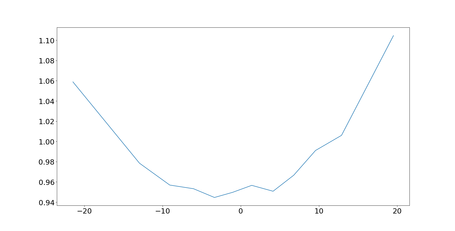
Finally let's return to the problem of non linear forecast response, 'reversion in the wings' for slower momentum. If we use our updated vol forecast, accounting for mean reversion, does it go away?
Here's a repeat of the plot from last time round, where I'm looking at the out turn of risk adjusted return versus forecast, for ewmac64_256 without capping. The blue line shows the original plot, and the orange line shows the data with an improved forecast using a blend of slow and current vol:
 |
| Forecast accuracy conditioned on risk adjusted return forecast values, without capping. Rule 'ewmac64_256', data summed across all instruments. X-axis: forecast value adjusted for vol forecast, Y-axis: risk adjusted return over holding period. Forecast for vol uses current vol and 10 year vol. Risk adjusted trading rule forecasts modified to reflect change in vol measure. |
 |
| Forecast accuracy conditioned on risk adjusted return forecast values, with capping. Rule 'ewmac64_256', data summed across all instruments. X-axis: forecast value adjusted for vol forecast, Y-axis: risk adjusted return over holding period. Forecast for vol uses current vol and 10 year vol. Risk adjusted trading rule forecasts modified to reflect change in vol measure. |
Hi Rob,
ReplyDeletevery interesting post!
So it seems that there is indeed a mean reversion effect in the volatility, but even once you account for it the forecast do not change significantly.
However, I do not think this post is a failure: in your system volatility is used directly for position sizing and overall risk management, so a more robust estimate should make the system safer (especially if one uses constant forecasts). Am I correct?
Also: in the scatter plot there's an interesting hole when vol gets quite high. It looks like in those conditions the vol forecast should be binary, if I'm reading the plot correctly (although there's little data to support this). As this seems an effect that arises when vol is relatively high and most of the data points are on the bottom left part of the curve, would it make sense to cap the estimate of vol as well?
"a more robust estimate should make the system safer (especially if one uses constant forecasts). Am I correct?" I certainly think so.
DeleteI really wouldn't draw too much inference from the scatter plot especially as it is just one market. A more accurate statement is that when vol is high, the dispersion of vol forecasting accuracy is probably also higher.
An interesting question is whether the rest of the market is using a similar enough signal that crowding becomes apt at a high level of forecast, and if there's a way to suss out whether such is an explanation for the nonlinearities in ex-post risk adjusted returns vs ex-ante signal.
ReplyDeleteThat is a very interesting question, and probably quite hard to answer. In fact it's probably easier to treat the non linearity as some kind of proxy for telling you when the trade is becoming overcrowded, and act accordingly.
DeleteHi Robert,
ReplyDeleteI couldn't get the above graphs. Is there anywhere that I can download the full codes pertaining to the blog's posts?
No I don't do that as it means even more code I have to maintain
DeleteThanks Rob, the past 2 posts were definitely an interesting and worthwhile investigation.
ReplyDeleteI prefer a forecast capping strategy, but have also seen smoothing function f(x) = (x*exp(-.25x^2))/(exp(-.5)*sqrt(2)) in literature. I suspect the optimal strategy is somewhere in between and also dependent on trading rule and asset.
Another thought is that it can be shown that the resulting return distribution per trade becomes more normal/less skewed for greater magnitude of momentum signal. Although this doesn’t explain why the mean flattens out, it might provide the rationale for limiting or reducing position size in order to maintain the desirable overall positive skew of the strategy.
Thanks Matt, I was aware of the formula you mentioned, but I hadn't given much thought to how skew changes in the outer regions of the forecast.
Delete