Lots of things have changed in the last year. Many unthinkable things are now thinkable. A war in Europe. The UK coming 2nd in the Eurovision song contest rather than the usual dismal 'null points'. And of course, the correlation of stocks and bonds has recently gone more positive than it has been for over 20 years:

I thought it would be 'fun' to see how the optimal stock/bond portfolio is affected by correlation and expected return assumptions.
In my second book, Smart Portfolios, I noted that a 100% equity portfolio made no sense under the Kelly criteria (AKA maximising CAGR), and that pretty much everyone should have some exposure to bonds regardless of their risk tolerance, even though they will have a lower expected arithmetic return due to their lower risk. For a while my own strategic risk weighting has been 10% in bonds, equating to cash weights of around 80/20.
I am currently reviewing my long only portfolio and it seems as good a time as any to check that 80/20 still makes sense.
Simple python code is liberally scattered throughout.
Assumptions and base case
I'm assuming a two asset, fully invested portfolio with two assets: a global stock, and a global bond (including both government and corporates). Both assets are Gaussian normal and have a linear relationship, so I can use an approximation for geometric return.
I assume that the standard deviation of the stocks is around 20% and the bonds around 10% (it's gone up recently, can't think why). Furthermore, I assume that my central case for the expected return in stocks is around 8%, and 5% in bonds. That corresponds to a simple SR (without risk free rate) of 0.4 and 0.5 respectively; eg a SR advantage for bonds versus the average SR of 0.05.
(Real return expectations are taken from AQR plus an assumed 3% inflation)
My utility function is to maximise real CAGR, which in itself implies I will be fully invested. Note that means I will be at 'full Kelly' - something that isn't usually advised. However we're determining allocations here, not leverage, so it's probably not as dangerous as you might think.
import numpy as np
import pandas as pd


def calculate_cagr(
    correlation, equity_weight, mean_eq, mean_bo, stdev_eq=0.2, stdev_bo=0.1
):
    bond_weight = 1 - equity_weight
    mean_return = (equity_weight * mean_eq) + (bond_weight * mean_bo)
    variance = (
        ((equity_weight**2) * (stdev_eq**2))
        + ((bond_weight**2) * (stdev_bo**2))
        + 2 * bond_weight * equity_weight * stdev_bo * stdev_eq * correlation
    )

    approx_cagr = mean_return - 0.5 * variance

    return approx_cagr
Effect of correlation varying with base case assumptions
I'm going to vary the correlation between stocks and bonds, between -0.8 and +0.8
list_of_weight_indices = list(np.arange(0, 1, 0.001))def iterate_cagr(correlation, mean_eq, mean_bo):
cagr_list = [
calculate_cagr(
correlation=correlation,
equity_weight=equity_weight,
mean_bo=mean_bo,
mean_eq=mean_eq,
)
for equity_weight in list_of_weight_indices
]
return cagr_list
corr_list = list(np.arange(-0.8, 0.8, 0.1))
corr_list = [round(x, 1) for x in corr_list]
## plot correlation varying
results = dict(
[(correlation, iterate_cagr(correlation, 0.08, 0.05)) for correlation in corr_list]
)
results = pd.DataFrame(results)
results.columns = corr_list
results.index = list_of_weight_indicesresults.plot()
def weight_with_max_cagr(correlation, mean_eq, mean_bo):
    cagr_list = iterate_cagr(correlation, mean_eq, mean_bo)
    max_cagr = np.max(cagr_list)
    index_of_max = cagr_list.index(max_cagr)
    wt_of_max = list_of_weight_indices[index_of_max]

    return wt_of_max


results = pd.Series(
    [weight_with_max_cagr(correlation, 0.08, 0.05) for correlation in corr_list],
    index=corr_list,
)

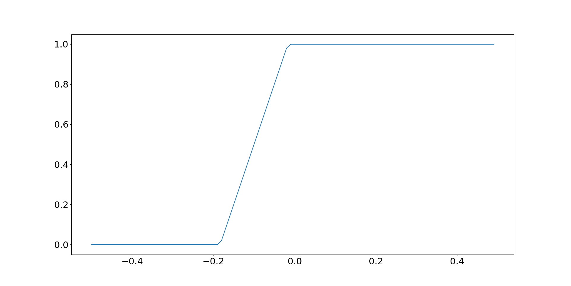
Effect of SR varying
def means_from_sr_diff(sr_diff, avg_sr=0.45, stdev_eq=0.2, stdev_bo=0.1):
    ## higher sr_diff is better for equities
    sr_eq = avg_sr + sr_diff
    sr_bo = avg_sr - sr_diff

    mean_eq = sr_eq * stdev_eq
    mean_bo = sr_bo * stdev_bo

    return mean_eq, mean_bo


def weight_with_max_cagr_given_sr_diff(correlation, sr_diff):
    mean_eq, mean_bo = means_from_sr_diff(sr_diff)
    return weight_with_max_cagr(correlation, mean_eq, mean_bo)


# fix corr at zero
sr_diff_list = list(np.arange(-0.5, 0.5, 0.01))
results = pd.Series(
    [weight_with_max_cagr_given_sr_diff(0, sr_diff) for sr_diff in sr_diff_list],
    index=sr_diff_list,
)
Effect of SR and correlations varying
sr_diff_list = list(np.arange(-0.25, 0.0501, 0.05))
sr_diff_list = [sr_diff.round(2) for sr_diff in sr_diff_list]
results = pd.DataFrame(
    dict(
        [
            (
                correlation,
                [
                    weight_with_max_cagr_given_sr_diff(correlation, sr_diff)
                    for sr_diff in sr_diff_list
                ],
            )
            for correlation in corr_list
        ]
    )
)

results.index = sr_diff_list
results.columns = corr_list
results = results.transpose()
results.plot()
Sensitivity
results = []
for correlation in [-0.4, 0, 0.4]:
    for sr_diff in [-0.25, 0, 0.25]:
        cagr80 = cagr_with_sr_diff(0.8, correlation, sr_diff)
        cagr90 = cagr_with_sr_diff(0.9, correlation, sr_diff)
        cagr100 = cagr_with_sr_diff(1, correlation, sr_diff)
        loss80 = cagr100 - cagr80
        loss90 = cagr100 - cagr90
        results.append(
            dict(
                correlation=correlation,
                sr_diff=sr_diff,
                cagr100=round(cagr100 * 100, 1),
                cagr90=round(cagr90 * 100, 1),
                cagr80=round(cagr80 * 100, 1),
                loss80=round(loss80 * 100, 2),
                loss90=round(loss90 * 100, 2),
            )
        )

print(pd.DataFrame(results))
  correlation  sr_diff  cagr100  cagr90  cagr80  loss80  loss90
0         -0.4    -0.25      2.0     2.7     3.4   -1.43   -0.75
1         -0.4     0.00      7.0     7.0     6.9    0.07    0.00
2         -0.4     0.25     12.0    11.2    10.4    1.57    0.75
3          0.0    -0.25      2.0     2.7     3.3   -1.30   -0.68
4          0.0     0.00      7.0     6.9     6.8    0.20    0.07
5          0.0     0.25     12.0    11.2    10.3    1.70    0.82
6          0.4    -0.25      2.0     2.6     3.2   -1.17   -0.60
7          0.4     0.00      7.0     6.9     6.7    0.33    0.15
8          0.4     0.25     12.0    11.1    10.2    1.83    0.90
This makes sense if only stocks and bonds are part of your investment universe. But if correlations have risen (and you're saying implicitly that they're expected to stay high) couldn't you consider other assets that could be part of a diversified portfolio (gold, commodities, inflation-linked bonds etc)?
ReplyDeleteOh sure but it's hard to draw these pretty plots with more than two assets. For a longer answer to your question, https://www.aqr.com/About-Us/News/2022/Press-Release or https://www.systematicmoney.org/smart
DeleteI'm sure you have considered a levered stocks/bonds/commodities risk parity allocation as an alternative to a mostly equity based portfolio. What are the reasons you went with the second solution? I guess one factor could be you don't want to use leverage since you already use it in your futures strategy?
DeleteThat's part of it. Also, about half my investments are in tax sheltered accounts where I can't trade futures. I also find it psychologically easier to use dividends from long only investments as income, rather than withdrawing from a futures account.
Delete