Monday, 14 November 2022

If you're so smart, how come you're not SBF? The Kelly criterion and choice of expectations and utility function when bet sizing


There has been a very interesting discussion on twitter, relating to some stuff said by Sam Bankman-Fried (SBF), who at the time of writing has just completely vaporized billions of dollars in record time via the medium of his crypto exchange FTX, and provided a useful example to future school children of the meaning of the phrase nominative determinism*.

* Sam, Bank Man: Fried. Geddit? 

Read the whole thread from the top:

https://twitter.com/breakingthemark/status/1591114381508558849

TLDR the views of SBF can be summarised as follows:

  • Kelly criterion maximises log utility
  • I don't have a log utility function. It's probably closer to linear.
  • Therefore I should bet at higher than Kelly. Up to 5x would be just fine.
I, and many others, have pointed out that SBF is an idiot. Of course it's easier to do this when he's just proven his business incompetence on a grand scale, but to be fair I was barely aware of the guy until a week ago. Specifically, he's wrong about the chain of reasoning above*. 

* It's unclear whether this is specifically what brought SBF down. At the time of writing he appears to have taken money from his exchange to prop up his hedge fund, so maybe the hedge fund was using >>> Kelly leverage, and this really is the case. 

In this post I will explain why he was wrong, with pictures. To be clearer, I'll discuss how the choice of expectation and utility function affects optimal bet sizing. 

I've discussed parts of this subject briefly before, but you don't need to read the previous post.


Scope and assumptions


To keep it tight, and relevant to finance, this post will ignore arguments seen on twitter related to one off bets, and whether you should bet differently if you are considering your contribution to society as a whole. These are mostly philosophical discussions which it's hard to solve with pictures. So the set up we have is:

  • There is an arbitrary investment strategy, which I assume consists of a data generating process (DGP) producing Gaussian returns with a known mean and standard deviation (this ignores parameter uncertainty, which I've banged on about often enough, but effectively would result in even lower bet sizing).
  • We make a decision as to how much of our capital we allocate to this strategy for an investment horizon of some arbitrary number of years, let's say ten.
  • We're optimising L, the leverage factor, where L =1 would be full investment, 2 would be 100% leverage, 0.5 would be 50% in cash 50% in the strategy and so on.
  • We're interested in maximising the expectation of f(terminal wealth) after ten years, where f is our utility function.
  • Because we're measuring expectations, we generate a series of possible future outcomes based on the DGP and take the expectation over those.
Note that I'm using the contionous version of the Kelly criterion here, but the results would be equally valid for the sort of discrete bets that appear in the original discussion.


Specific parameters

Let's take a specific example. Set mean =10% and standard deviation = 20%, which is a Sharpe ratio of 0.5, and therefore Kelly should be maxed at 50% risk, equating to L = 50/20 = 2.5. SBF optimal leverage would be around 5 times that, L = 12.5. We start with wealth of 1 unit, and compound it over 10 years.

I don't normally paste huge chunks of code in these blog posts, but this is a fairly short chunk:

import pandas as pd
import numpy as np
from math import log

ann_return = 0.1
ann_std_dev = 0.2

BUSINESS_DAYS_IN_YEAR = 256
daily_return = ann_return / BUSINESS_DAYS_IN_YEAR
daily_std_dev = ann_std_dev / (BUSINESS_DAYS_IN_YEAR**.5)

years = 10
number_days = years * BUSINESS_DAYS_IN_YEAR


def get_series_of_final_account_values(monte_return_streams,
leverage_factor = 1):
account_values = [account_value_from_returns(returns,
leverage_factor=leverage_factor)
for returns in monte_return_streams]

return account_values

def get_monte_return_streams():
monte_return_streams = [get_return_stream() for __ in range(10000)]

return monte_return_streams

def get_return_stream():
return np.random.normal(daily_return,
daily_std_dev,
number_days)

def account_value_from_returns(returns, leverage_factor: float = 1.0):
one_plus_return = np.array(
[1+(return_item*leverage_factor)
for return_item in returns])
cum_return = one_plus_return.cumprod()

return cum_return[-1]

monte_return_streams = get_monte_return_streams()

Utility function: Expected log(wealth) [Kelly]

Kelly first. We want to maximise the expected log final wealth:

def expected_log_value(monte_return_streams,
leverage_factor = 1):

series_of_account_values =get_series_of_final_account_values(
monte_return_streams = monte_return_streams,
leverage_factor = leverage_factor)
log_values_over_account_values = [log(account_value) for account_value in series_of_account_values]

return np.mean(log_values_over_account_values)

And let's plot the results:

def plot_over_leverage(monte_return_streams, value_function):
leverage_ratios = np.arange(1.5, 5.1, 0.1)
values = []
for leverage in leverage_ratios:
print(leverage)
values.append(
value_function(monte_return_streams, leverage_factor=leverage)
)

leverage_to_plot = pd.Series(
values, index = leverage_ratios
)

return leverage_to_plot

leverage_to_plot = plot_over_leverage(monte_return_streams,
expected_log_value)
leverage_to_plot.plot()

In this plot, and nearly all of those to come, the x-axis shows the leverage L and the y-axis shows the value of the expected utility. To find the optimal L we look to see where the highest point of the utility curve is.

As we'd expect:

  • Max expected log(wealth) is at L=2.5. This is the optimal Kelly leverage factor.
  • At twice optimal we expect to have log wealth of zero, equivalent to making no money at all (since starting wealth is 1).
  • Not plotted here, but at SBF leverage (12.5) we'd have expected log(wealth) of <undefined> and have lost pretty much all of our money.


Utility function: Expected (wealth) [SBF?]

Now let's look at a linear utility function, since SBF noted that his utility was 'roughly close to linear'. Here our utility is just equal to our terminal wealth, so it's purely linear.

def expected_value(monte_return_streams,
leverage_factor = 1):

series_of_account_values =get_series_of_final_account_values(
monte_return_streams = monte_return_streams,
leverage_factor = leverage_factor)

return np.mean(series_of_account_values)
leverage_to_plot = plot_over_leverage(monte_return_streams,
expected_value)

You can see where SBF was coming from, right? Utility gets exponentially higher and higher, as we add more leverage. Five times leverage is a lot better than 2.5 times, the Kelly criterion. Five times Kelly, or 2.5 * 5= 12.5, would be even better.


Utility function: Median(wealth) 

However there is an important assumption above, which is the use of the mean for the expectation operator. This is dumb. It would mean (pun, sorry), for example, that of the following:

  1. An investment that lost $1,000 99 times out of 100; and paid out $1,000,000 1% of the time
  2. An investment that is guaranteed to gain $9,000 

... we would theoretically prefer option 1 since it has an expected value of $9,010, higher than the trivial expected value of $9,000 for option 2. There might be some degenerate gamblers who prefer 1 to 2, but not many.

(Your wealth would also affect which of these you would prefer. If $1,000 is a relatively trivial amount to you, you might prefer 1. If this is the case consider if you'd still prefer 1 to 2 if the figures were 1000 times larger, or a million times larger). 

I've discussed this before, but I think the median is the more appropriate. What the median implies in this context is something like this: 

Considering all possible future outcomes, how can I maximise the utility I receive in the outcome that will occur half the time?

I note that the median of option 1 above is zero, whilst the median of option 2 is $9,000. Option 2 is now far more attractive.


def median_value(monte_return_streams,
leverage_factor = 1):

series_of_account_values =get_series_of_final_account_values(
monte_return_streams = monte_return_streams,
leverage_factor = leverage_factor)

return np.median(series_of_account_values)


The spooky result here is that the optimal leverage is now 2.5, the same as the Kelly criterion.

Even with linear utility, if we use the median expectation, Kelly is the optimal strategy.

The reason why people prefer to use mean(log(wealth)) rather than median(wealth), even though they are equivalent, is that the former is more computationally attractive.

Note also the well known fact that Kelly also maximises the geometric return.

With Kelly we aren't really making any assumptions about utility function: our assumption is effectively that the median is the correct expectations operator

The entire discussion about utility is really a red herring. It's very hard to measure utility functions, and everyone probably does have a different one, I think it's much better to focus on expectations.


Utility function: Nth percentile(wealth) 

Well you might be thinking that SBF seems like a particularly optimistic kind of guy. He isn't interested in the median outcome (which is the 50% percentile). Surely there must be some percentile at which it makes sense to bet 5 times Kelly? Maybe he is interested in the 75% percentile outcome?

QUANTILE = .75
def value_quantile(monte_return_streams,
leverage_factor = 1):

series_of_account_values =get_series_of_final_account_values(
monte_return_streams = monte_return_streams,
leverage_factor = leverage_factor)

return np.quantile(series_of_account_values, QUANTILE)

Now the optimal is around L=3.5. This is considerably higher than the Kelly max of L=2.5, but it is still nowhere near the SBF optimal L of 12.5.

Let's plot the utility curves for a bunch of different quantile points:

list_over_quantiles = []
quantile_ranges = np.arange(.4, 0.91, .1)
for QUANTILE in quantile_ranges:
leverage_to_plot = plot_over_leverage(monte_return_streams,
value_quantile)
list_over_quantiles.append(leverage_to_plot)

pd_list = pd.DataFrame(list_over_quantiles)
pd_list.index = quantile_ranges
pd_list.transpose().plot()

It's hard to see what's going on here, legend floating point representation notwithstanding, but you can hopefully see that the maximum L (hump of each curve) gets higher as we go up the quantile scale, as the curves themselves get higher (as you would expect).

But in none of these quantiles we are still nowhere near reaching an optimal L of 12.5. Even at the 90% quantile - evaluating something that only happens one in ten times - we have a maximum L of under 4.5.

Now there will be some quantile point at which L=12.5 is indeed optimal. Returning to my simple example:

  1. An investment that lost $1,000 99 times out of 100; and paid out $1,000,000 1% of the time
  2. An investment that is guaranteed to gain $9,000 

... if we focus on outcomes that will happen less than one in a million times (the 99.9999% quantile and above) then yes sure, we'd prefer option 1.

So at what quantile point does a leverage factor of 12.5 become optimal? I couldn't find out exactly, since to look at extremely rare quantile points requires very large numbers of outcomes*. I actually broke my laptop before I could work out what the quantile point was. 

* for example, if you want ten observations to accurately measure the quintile point, then for the 99.99% quantile you would need 10* (1/(1-0.9999)) = 100,000 outcomes.

But even for a quantile of 99.99% (!), we still aren't at an optimal leverage of 12.5! 


You can see that the optimal leverage is 8 (around 3.2 x Kelly), still way short of 12.5.


Summary

Rather than utility functions, I think it's easier to say to ask people the likelihood of outcome they are concerned about. I'd argue that sensible people would think about the median outcome, which is what you expect to happen 50% of the time. And if you are a bit risk averse, you should probably consider an even lower quantile. 

In contrast SBF went for bet sizing that would only make sense in the set of outcomes that happens significantly less than 0.01% of the time. That is insanely optimistic; and given he was dealing with billions of dollars of other peoples money it was also insanely irresponsible.

Was SBF really that recklessly optimistic, or dumb? In this particular case I'd argue the latter. He had a very superfical understanding of Kelly bet sizing, and because of that he thought he could ignore it. 
This is a classic example of 'a little knowledge is a dangerous thing'. A dumb person doesn't understand anything, but reads on the internet somewhere that half Kelly is the correct bet sizing. So they use it. A "smart" person like SBF glances at the Kelly formula, thinks 'oh but I don't have log utility' and leverages up five times Kelly and thinks 'Wow I am so smart look at all my money'. And that ended well...

A truely enlightened person understands that it isn't about the utility function, but about the expectation operator. They also understand about uncertainty, optimistic backtesting bias, and a whole bunch of factors that imply that even 0.5 x Kelly is a little reckless. I, for example, use something south of a quarter Kelly. 

Which brings us back to the meme at the start of the post:


Note I am not saying I am smarter than SBF. On pure IQ, I am almost certainly much, much dumber. In fact, it's because I know I am not a genius that I'm not arrogant enough to completely follow or ignore the Kelly criteria without first truely understanding it.

Whilst this particular misunderstanding might not have brought down SBF's empire, it shows that really really smart people can be really dumb - particularly when they think that they are so smart they don't need to properly understand something before ignoring it*.

* Here is another example of him getting something completely wrong


Postscript (16th November 2022)

I had some interesting feedback from Edwin Teejay on twitter, which is worth addressing here as well. Some of the feedback I've incorporated into the post already.

(Incidentally, Edwin is a disciple of Ergodic Economics, which has a lot of very interesting stuff to say about the entire problem of utility maximisation)

First he commented that the max(median) = max(log) relationship is only true for a long sequence of bets, i.e. asymptotically. We effectively have 5000 bets in our ten year return sequence. As I said originally, I framed this as a typical asset optimisation problem rather than a one off bet (or small number of one off bets).

He then gives an example of a one off bet decision where the median would be inappropriate:
  1. 100% win $1
  2. 51% win $0 / 49% win $1'000'000
The expected values (mean expectation) are $1 and $490,000 respectively, but the medians are $1 and $0. But any sane person would pick the second option.

My retort to this is essentially the same as before - this isn't something that could realistically happen in a long sequence of bets. Suppose we are presented with making the bet above every single week for 5 weeks. The distribution of wealth outcomes for option 1 is single peaked - we earn $5. The distribution of wealth outcomes for option 2 will vary from $0 (with probability 3.4%) to $5,000,000 (with a slightly lower probability of 2.8% - I am ignoring 'compounding', eg the possibility to buy more bets with money we've already won), with a mean of $2.45 million. 

But the median is pretty good: $1 million. So we'd definitely pick option 2. And that is with just 5 bets in the sequence. So the moment we are looking at any kind of repeating bet, the law of large numbers gets us closer and closer to the median being the optimal decision. We are just extremely unlikely to see the sort of payoff structure in the bet shown in a series of repeated bets.

Now what about the example I posted:
  1. An investment that lost $1,000 99 times out of 100; and paid out $1,000,000 1% of the time
  2. An investment that is guaranteed to gain $9,000 
Is it realistic to expect this kind of payoff structure in a series of repeated bets? Well consider instead the following:
  1. An investment that lost $1 most of the time; and paid out $1,000,000 0.001% of the time
  2. An investment that is guaranteed to gain $5

The mean of these bets is ~$9 and $5, and the medians are $-1 and $5.

Is this unrealistic? Well, these sorts of payoffs do exist in the world- they are called lottery tickets (albeit it is rare to get a lottery ticket with a $9 positive mean!). And this is something closer to the SBF example, since I noted that he would have to be looking at somewhere north of the 0.01% quantile to choose 5x Kelly Leverage.

Now what happens if we run the above as a series of 5000 repeated bets (again with no compounding for simplicity).  We end up with the following distributions:
  1. An investment that lost $5000 95.1% of the time, and makes $1 million or more 5% of the time.
  2. An investment that is guaranteed to gain $25,000

Since there is no compounding we can just multiply up the individual numbers to get the mean ($45,000  and $25,000 respectively). The medians are -$5,000 and $25,000. Personally, I still prefer option 2! You might still prefer option 2 if spending $5,000 on lottery tickets over 10 years reflects a small proportion of your wealth, but I refer you to the previous discussion on this topi: make 

So I would argue that it in a long run of bets we are more likely in real life to get payoff structures of the kind I posited, than the closer to 50:50 bet suggested by Edwin. Ultimately, I think we agree that for long sequences of bets the median makes more sense (with a caveat). I personally think long run decision making is more relevant to most people than one off bets. 

What is the caveat? Edwin also said that the choice of the median is 'arbitrary'. I disagree here. The median is 'what happens half the time'. I still think for most people that is a logical reference point for 'what I expect to happen', as well as in terms of the maths: both median and mean are averages after all. I personally think it's fine to be more conservative than this if you are risk averse, but not to be more aggressive - bear in mind that will mean you are betting at more than Kelly.

But anyway, as Matt Hollerbach, whose orginal series of tweets inspired this post, said:

"The best part of Robs framework is you don't have to use the median,50%. You could use 60%  or 70%  or 40% if your more conservative.  And it intuitively tells you what the chance of reaching your goal is. You don't get duped into a crazy long shot that the mean might be hiding in."  (typos corrected from original tweet)

This fits well into my general framework for thinking about uncertainty. Quantify it, and be aware of it. Then if you still do something crazy/stupid, well at least you know you're being an idiot...


Wednesday, 2 November 2022

Optimal trend following allocation under conditions of uncertainty and without secular trends

Few people are brave enough to put their entire net worth into a CTA fund or home grown trend following strategy (my fellow co-host on the TTU podcast, Jerry Parker, being an honorable exception with his 'Trend following plus nothing' portfolio allocation strategy). Most people have considerably less than 100% - and I include myself firmly in that category. And it's probably true that most people have less than the sort of optimal allocation that is recommended by portfolio optimisation engines.

Still it is a useful exercise to think about just how much we should allocate to trend following, at least in theory. The figure that comes out of such an exercise will serve as both a ceiling (you probably don't want any more than this), and a target (you should be aiming for this). 

However any sort of portfolio optimisation based on historical returns is likely to be deeply flawed. I've covered the problems involved at length before, in particular in my second book and in this blogpost, but here's a quick recap:

  1. Standard portfolio optimisation techniques are not very robust
  2. We often assume normal distributions, but financial returns are famously abnormal
  3. There is uncertainty in the parameter estimates we make from the data
  4. Past returns distributions may be biased and unlikely to repeat in the future

As an example of the final effect, consider the historically strong performance of equities and bonds in a 60:40 style portfolio during my own lifetime, at least until 2022. Do we expect such a performance to be repeated? Given it was driven by a secular fall in inflation from high double digits, and a resulting fall in interest rates and equity discount rates, probably not. 

Importantly, a regime change to lower bond and equity returns will have varying impact on a 60:40 long only portfolio (which will get hammered), a slow trend following strategy (which will suffer a little), and a fast trend following strategy (which will hardly be affected). 

Consider also the second issue: non Gaussian return distributions. In particular equities have famously negative skew, whilst trend following - especially the speedier variation - is somewhat positive in this respect. Since skew affects optimal leverage, we can potentially 'eat' extra skew in the form of higher leverage and returns. 

In conclusion then, some of the problems of portfolio optimisation are likely to be especially toxic when we're looking at blends of standard long only assets combined with trend following. In this post I'll consider some tricks methods we can use to alleviate these problems, and thus come up with a sensible suggestion for allocating to trend following. 

If nothing else, this is a nice toy model for considering the issues we have when optimising, something I've written about at length eg here. So even if you don't care about this problem, you'll find some interesting ways to think about robust portfolio optimisation within.

Credit: This post was inspired by this tweet.

Some very messy code with hardcoding galore, is here.


The assets

Let's first consider the assets we have at our disposal. I'm going to make this a very simple setup so we can focus on what is important whilst still learning some interesting lessons. For reasons that will become apparent later, I'm limiting myself to 3 assets. We have to decide how much to allocate to each of the following three assets:

  • A 60:40 long only portfolio of bonds and equities, represented by the US 10 year and S&P 500
  • A slow/medium speed trend following strategy, trading the US 10 year and S&P 500 future with equal risk allocation, with a 12% equity-like annualised risk target. This is a combination of EWMAC crossovers: 32,128 and 64,256
  • A relatively fast trend following strategy, trading the US 10 year and S&P 500 future with equal risk allocation, with a 12% annualised risk target. Again this is a combination of EWMAC crossovers: 8, 32 and 16,64

Now there is a lot to argue with here. I've already explained why I want to allocate seperately to fast and slow trend following; as it will highlight the effect of secular trends.

The reason for the relatively low standard deviation target is that I'm going to use a non risk adjusted measure of returns, and if I used a more typical CTA style risk (25%) it would produce results that are harder to interpret.

You may also ask why I don't have any commodities in my trend following fund. But what I find especially interesting here is the effect on correlations between these kinds of strategies when we adjust for long term secular trends. These correlations will be dampened if there are other instruments in the pot. The implication of this is that the allocation to a properly diversified trend following fund running futures across multiple asset classes will likely be higher than what is shown here.

Why 60:40? Rather than 60:40, I could directly try and work out the optimal allocation to a universe of bonds and equities seperately. But I'm taking this as exogenous, just to simplify things. Since I'm going to demean equity and bond returns in a similar way, this shouldn't affect their relative weightings.

50:50 risk weights on the mini trend following strategies is more defensible; again I'm using fixed weights here to make things easier and more interpretable. For what it's worth the allocation within trend following for an in sample backtest would be higher for bonds than for equities, and this is especially true for the faster trading strategy.

Ultimately three assets makes the problem both tractable and intuitive to solve, whilst giving us plenty of insight.


Characteristics of the underyling data

Note I am going to use futures data even for my 60:40, which means all the returns I'm using are excess returns.

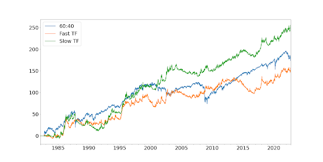
Let's start with a nice picture:


So the first thing to note is that the vol of the 60:40 is fairly low at around 12%; as you'd expect given it has a chunky allocation to bonds (vol ~6.4%). In particular, check out the beautifully smooth run from 2009 to 2022. The two trading strategies also come in around the 12% annualised vol mark, by design. In terms of Sharpe Ratio, the relative figures are 0.31 (fast trading strategy), 0.38 (long only) and 0.49 (slow trading strategy). However as I've already noted, the performance of the long only and slow strategies is likely to be flattered by the secular trends in equities and bonds seen since 1982 (when the backtest starts).

Correlations matter, so here they are:

         60:40  Fast TF  Slow TF
60:40 1.00 -0.02 0.25
Fast TF -0.02 1.00 0.68
Slow TF 0.25 0.68 1.00

What about higher moments? The monthly skews are -1.44 (long only), 0.08 (slow) and 0.80 (fast). Finally what about the tails? I have a novel method for measuring these which I discuss in my new book, but all you need to know is that a figure greater than one indicates a non-normal distribution. The lower tail ratios are 1.26 (fast), 1.35 (slow) and 2.04 (long only); whilst the uppers are 1.91 (fast), 1.74 (slow) and 1.53 (long only). In other words, the long only strategy has nastier skew and worst tails than the fast trading strategy, whilst the slow strategy comes somewhere in between.


Demeaning

To reiterate, again, the performance of the long only and slow strategies is likely to be flattered by the secular trends in equities and bonds, caused by valuation rerating in equities and falling interest rates in bonds. 

Lets take equities. The P/E ratio in September 1982 was around 9.0, versus 20.1 now. This equates to 2.0% a year in returns coming from the rerating of equities. Over the same period US 10 year bond yields have fallen from around 10.2% to 4.0% now, equating to around 1.2% a year in returns. I can do a simple demeaning to reduce the returns achieved by the appropriate amounts.

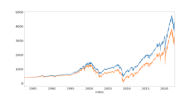
Here are the demeaned series with the original backadjusted prices. First S&P:

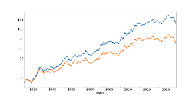
And for US10:


What effect does the demeaning have? It doesn't affect significantly standard deviations, skew, or tail ratios. But it does affect the Sharpe Ratio:


              Original       Demean     Difference

Long only       0.38          0.24        -0.14

Slow TF         0.49          0.41        -0.08

Fast TF         0.31          0.25        -0.06

This is exactly what we would expect. The demeaning has a larger effect on the long only 60:40, and to a lesser extent the slower trend following. 

And the correlation is also a little different:

         60:40  Fast TF  Slow TF
60:40 1.00 -0.06 0.18
Fast TF -0.06 1.00 0.66
Slow TF 0.18 0.66 1.00

Both types of trend have become slightly less correlated with 60:40, which makes sense.


The optimisation

Any optimisation requires (a) a utility or fitness function that we are maximising, and (b) a method for finding the highest value of that function. In terms of (b) we should bear in mind the comments I made earlier about robustness, but let's first think about (a).

An important question here is whether we should be targeting a risk adjusted measure like Sharpe Ratio, and hence assuming leverage is freely available, which is what I normally do. But for an exercise like this a more appropriate utility function will target outright return and assume we can't access leverage. Hence our portfolio weights will need to sum to exactly 100% (we don't force this to allow for the possibility of holding cash; though this is unlikely). 

It's more correct to use geometric return, also known as CAGR, rather than arithmetic mean since that is effectively the same as maximising the (log) final value of your portfolio (Kelly criteria). Using geometric mean also means that negative skew and high kurtosis strategies will be punished, as will excessive standard deviation. By assuming a CAGR maximiser, I don't need to worry about the efficient frontier, I can maximise for a single point. It's for this reason that I've created TF strategies with similar vol to 60:40.

I'll deal with uncertainty by using a resampling technique. Basically, I randomly sample with replacement from the joint distribution of daily returns for the three assets I'm optimising for, to create a new set of account curves (this will preserve correlations, but not autocorrelations. This would be problematic if I was using drawdown statistics, but I'm not). For a given set of instrument weights, I then measure the utility statistic (CAGR) for the resampled returns. I repeat this exercise a few times, and then I end up with a distribution of CAGR for a given set of weights. This allows us to take into account the effect of uncertainty. 

Finally we have the choice of optimisation technique. Given we have just three weights to play with, and only two degrees of freedom, it doesn't seem too heroic to use a simple grid search. So let's do that.


Some pretty pictures

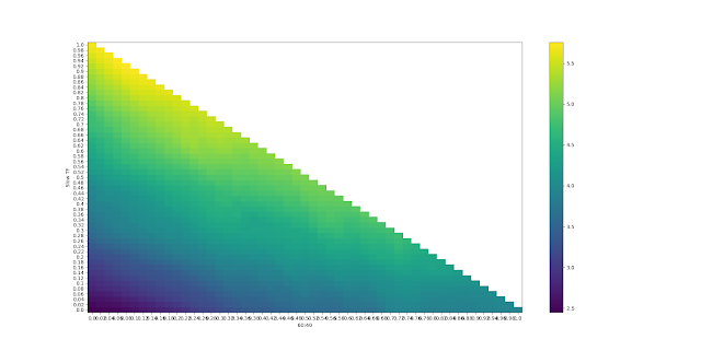
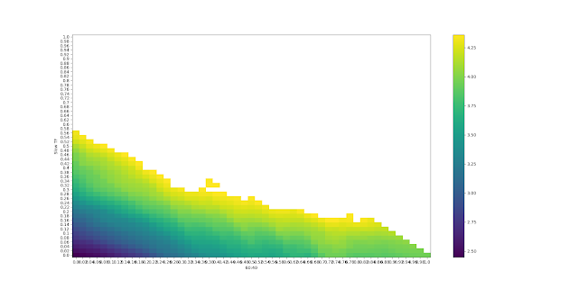
Because we only have two degrees of freedom, we can plot the results on a 2-d heatmap. Here's the results for the median CAGR, with the original set of returns before demeaning:
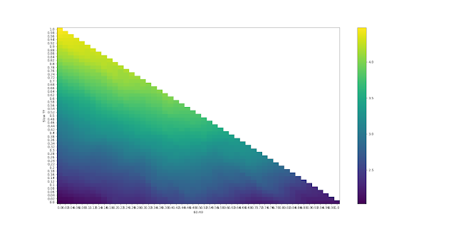
Sorry for the illegible labels - you might have to click on the plots to see them. The colour shown reflects the CAGR. The x-axis is the weight for the long only 60:40 portfolio, and the y-axis for slow trend following. The weight to fast trend following will be whatever is left over. The top diagonal isn't populated since that would require weights greater than 1; the diagonal line from top left to bottom right is where there is zero weight to fast trend following; top left is 100% slow TF and bottom right is 100% long only.

Ignoring uncertainty then, the optimal weight (brightest yellow) is 94% in slow TF and 6% in long only. More than most people have! However note that there is a fairly large range of yellow CAGR that are quite similar. 

The 30% quantile estimate for the optimal weights is a CAGR of 4.36, and for the 70% quantile it's 6.61. Let's say we'd be indifferent between any weights whose median CAGR falls in that range (in practice then, anything whose median CAGR is greater than 4.36). If I replace everything that is statistically indistinguishable from the maximum with white space, and redo the heatmap I get this:

This means that, for example, a weight of 30% in long only, 34% in slow trend following, and 36% in fast trend following; is just inside the whitespace and thus is statistically indistinguishable from the optimal set of weights. Perhaps of more interest, the maximum weight we can have to long only and still remain within this region (at the bottom left, just before the diagonal line reappears) is about 80%.

Implication: We should have at least 20% in trend following.

If I had to choose an optimal weight, I'd go for the centroid of the convex hull of the whitespace. I can't be bothered to code that up, but by eye it's at roughly 40% 60/40, 50% slow TF, 10% fast TF.

Now let's repeat this exercise with the secular trends removed from the data.

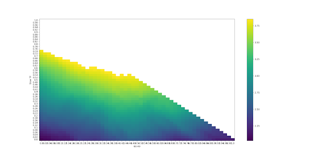
The plot is similar, but notice that the top left has got much better than the bottom right; we should have a lower weight to 60:40 than in the past. In fact the optimal is 100% in slow trend following; zilch, nil, zero, nada in both fast TF and 60:40.

But let's repeat the whitespace exercise to see how robust this result is:

The whitespace region is much smaller than before, and is heavily biased towards the top left. Valid portfolio weights that are indistinguishable from the maximum include 45% in 60:40 and 55% in slow TF (and 45% is the most you should have in 60:40 whilst remaining in this region). We've seen a shift away from long only (which we'd expect), but interestingly no shift towards fast TF, which we might have expected as it is less affected by demeaning.

The optimal (centroid, convex hull, yada yada...) is somewhere around 20% 60:40, 75% slow TF and 5% in fast TF.


Summary: practical implications

This has been a highly stylised exercise, deliberately designed to shine a light on some interesting facts and show you some interesting ways to visualise the uncertainty in portfolio optimisation. You've hopefully seen how we need to consider uncertainty in optimisation, and I've shown you a nice intuitive way to produce robust weights.

The bottom line then is that a robust set of allocations would be something like 40% 60/40, 50% slow TF, 10% fast TF; but with a maximum allocation to 60/40 of about 80%. If we use data that has had past secular trends removed, we're looking at an even higher allocation to TF, with the maximum 60/40 allocation reducing considerably, to around 45%

Importantly, this has of course been an entirely in sample exercise. Although we've made an effort to make things more realistic by demeaning, much of the results depend on the finding that slow TF has a higher SR than 60:40, an advantage that is increased by demeaning. Correcting for this would result in a higher weight to 60:40, but also to fast TF.

Of course if we make this exercise more realistic, it will change these results:
  • Improving 60:40 equities- Introducing non US assets, and allocating to individual equities
  • Improving 60:40 bonds -  including more of the term structure, inflation and corporate bonds, 
  • Improving 60:40 by including other non TF alternatives
  • Improving the CTA offering - introducing a wider set of instruments across asset classes (there would also be a modest benefit from widening beyond a single type of trading rule)
  • Adding fees to the CTA offering 
I'd expect the net effect of these changes to result in a higher weight to TF, as the diversification benefits in going from two instruments to say 100 is considerable; and far outweights the effect of fees and improved diversification in the long only space.

Tuesday, 20 September 2022

What exactly is a CTA?

When I use a word... it means just what I choose it to mean


CTA. An industry standard term, that seems straightforward to define: Commodity Trading Advisor. We can all name a bunch of CTAs - I used to work for one. There are indices for them, such as this one or this one (also this, and this, oh and this, plus this, and these guys have one, as do these guys, oh and dont' forget this one ... I probably missed some but I'm bored now).  But in practice, the term CTA is a somewhat ill defined term with multiple overlapping meanings. Let's dive in.


Advising and managed accounts


The most intriguing word in the term CTA is the final one: advisor. CTA's are not fund managers in the normal sense of the word. 

Fund managers normally do this: They take your cash and comingle it with others in a legal vehicle, selling you shares in the vehicle in exchange. Then they go out and buy assets with the cash. You don't legally own the assets - the fund does. There's normally a second legal vehicle which is responsible for actually managing the fund - the fund manager. You don't own shares in that. 

The CTA is a bit like the second legal vehicle in a standard fund structure - it advises but doesn't actually own the assets. But in a traditional CTA structure the assets are not comingled but kept seperate. So it works as follows: you open a managed account and put some cash into it. The CTA fund then makes decisions about what that account buys or sells. Importantly, you still own the assets in the account. If something happened to another customers assets, it wouldn't affect you.

Note that the advisory term is a bit misleading as it implies that you have full trading discretion on the account, and the CTA ocasionally rings you up and advises you about what you might think about trading. That may have been the case in the 1970s when CTAs started to become popular, but nowadays CTAs almost always trade customers accounts for them, often with automated execution algos that are a world away from requiring someone to pick up the phone. 


Choice of instrument


In theory any asset can be put inside a managed account, but they have normally been used to trade futures. The combination of a managed account and futures trading brings us to the term managed futures which is often used interchangeably with the designation CTA. Since CTA is a term of US legal art, this definition is safer and can be used across geographical regions.

An important implication of this is that you need a fair bit of money to have a managed account. To hold a properly diversified portfolio of futures with anything less than a few tens of millions, without running into discretisation issues is tricky, as I've discussed at length on this blog. There are also admin and operational fixed costs associated with having a number of managed accounts.

Over time many CTAs have gradually increased the minimum required to hold managed accounts, or have switched to using non managed account structures, which also allow them to trade assets that aren't futures. 


The asset class 


You might think that commodity trading advisors manage commodities: things like Wheat and Crude Oil. The easiest way to manage such things, especially in a managed account type setup, is through futures contracts.

However it's pretty rare for a CTA to only trade commodity futures. Nearly all of them also trade financial futures like the S&P 500 equity index or US 10 year bonds (there's perhaps an argument about whether metals like Gold are commodities or not).

Over time, CTAs have begun to trade non futures instruments. For example, it's hard to get adequate diversification in FX with just the available futures contracts. Adding FX forwards makes a lot of sense in this context, as they are very similar to futures although obviously OTC rather than exchange traded. This has implications for the legal structure of the CTA, since you can't easily put these in managed accounts.


The legal / regulatory definition


CTA is a US regulatory term. From the horses mouth:

Commodity Trading Advisor (CTA) Registration

A commodity trading advisor (CTA) is an individual or organization that, for compensation or profit, advises others, directly or indirectly, as to the value of or the advisability of trading futures contracts, options on futures, retail off-exchange forex contracts or swaps.

There's quite a bit to unpick there. The most obvious is this: the advisor is expected to advise, suggesting a managed account structure rather than a traditional structure. Secondly, and contrary to what has been stated before, you can be a CTA and manage non futures assets. This is somewhat alien to the concept of managed futures, but reflects the reality of the modern CTA industry. 


Trading style and speed


Until now I haven't discussed exactly how the CTA trades, only what it trades, and the legal structure set up to do that trading. In theory a CTA could be anything from a high frequency futures trader, up to a slow moving risk parity fund. They could be doing pure trend following, or some dangerous combination of carry, mean reversion, and a systematic short position in VIX.

Generally though when people refer to CTAs or managed futures they are mostly expecting such funds to trade medium to slow speed trend following. This is pure path dependence and tradition - there is nothing in the CFTC or NFA definition that says you have to trade like this. But because CTAs have been around for a while, and because trading costs where higher in the past, and because trends work well in futures particularly during the inflation ridden era when CTAs came to prominence, and because trends work better for holding periods between a few months and a year... for all of these reasons the CTA industry grew up as fairly slow trend followers.

(Remarkably this is true of both the US and European 'wings' of the CTA industry; even though the latter grew up fairly independently.)

There is a degree of self reinforcement here. CTAs have done very well in several market downturns, leading to the mythical status of 'crisis alpha'; something that is both uncorrelated and yet provides a positive return, plus nice skew properties. Some of that is just maths - a trend following strategy will have the payoff function of a long straddle and positive skew when judged at the right time horizon - and some of it may be myth, luck, or due to secular trends and correlations that may not hold in the future. But as a marketing story it's certainly become popular in certain circles, which means that many clients expect CTAs to have a certain trading style to fit within their particular style box.

However the fact that there are now seperate 'SG CTA', 'SG CTA Trend', and 'SG Short term' CTA indices suggests there is now more to the industry than slothful trend followers.

Note: The HFRI index family does not use the term CTA, but does have the following confusing set of indices:

  • HFRI Macro: Systematic Diversified Index 
  • HFRI Macro: Systematic Directional Index 
  • HFRI Trend Following Directional Index 


Systematic or discretionary


The very first CTAs can really only have been discretionary; men (back then, always men!) in green eye shades in darkened rooms looking at point and figure charts. However the use of trend following naturally lends itself to a systematic process. Systematisation also allows maximal diversification across numerous futures instruments, something that will improve expected performance.

The term CTA has thus become synonymous with systematic trend following. 

Notice that systematic is not the same as automated. It's possible in theory to have a fully systematic process which is hand cranked, or done in spreadsheets or with a calculator. The original turtles operated in such a fashion. But the easy availability of computer power means that the generation of trades in the vast majority of CTAS is now done in an automated fashion.


The modern CTA


A modern CTA may well still have some legacy managed accounts, or accounts opened for particularly large clients who want that traditional structure, but they are more likely to have morphed into a more typical hedge fund setup.

Instead of opening a managed account clients will buy shares in various legal investment vehicles, and there is usually a good offering of alternative jurisdictions (both onshore and offshore), currencies and types of fund (eg UCITS). In many cases a single legal vehicle may have different share classes, offering different currencies or degrees of leverage. 

(Another possibility is that the CTA uses a master-feeder structure. The client puts money into a feeder, which in turn is invested in various master funds. For example, a CTA might offer a variety of options that blend between a more traditional futures trend following fund, and an alternative that holds OTC assets.) 

These various funds will then have futures accounts opened them. Arguably these are also managed accounts, but the legal owner of the assets within them are funds not the final clients, so this is different from the traditional setup. 

However the investment funds can also go out shopping for assets that aren't futures. These can include other on exchange assets, like options on futures, or equities; or OTC assets like FX forwards, interest rate swaps or cash bonds.  This gives the clients access to a more diviersified set of instruments, something that would be extremely difficult in a traditional managed account structure. Consider for example the hassle of setting up 50 ISDA agreements for 50 $20 million managed accounts, rather than a single $1 billion fund.

It's likely that a modern CTA is fully systematic and automated up to the point of trade generation, although many funds will outsource the execution of their trades to in house human traders or external brokers. 

The variety of trading strategies is probably the area where the industry remains most heterogeneous. 

Many CTAs probably still have some medium speed trend following at their core, and may offer funds that are purer, but will have plenty of other signals such as carry and mean reversion. They may also offer funds that are very different but leverage off their experience, such as leveraged risk parity or equity market neutral. But this is a generalisation, and there are plenty of CTAs that have stuck more to their traditional knitting of medium speed trend following "plus nothing". We can even have a further debate about what does, or does not, constitute the correct use of the word trend following - but perhaps we should not do that today!


Conclusion


In summary, when you say CTA you may mean something quite different from what I mean. There is no such thing as a 'pure' or 'true' CTA. This is most true when it comes to defining the trading style. CTA is a poorly defined term, but it seems we are stuck with it (after all, 'managed futures' is not much better!).


Monday, 27 June 2022

Vol targeting: A CA(g)R race

Regular listeners to the podcast I ocasionally co-host will know that I enjoy some light hearted banter with some of my fellow podcasters, many of whom describe themselves as 'pure' trend followers, whilst I am an apostate who deserves to be cast into the outer darkness. My (main) sin? The use of 'vol targeting', an evil methodology not to be found in the original texts of trend following, or even in the apocrypha, and thus making me unworthy. In brief, vol targeting involves adjusting the size of a trade if volatility changes during the period that you are holding it for. A real trend follower would maintain the position in the original size.

(But we agree that the initial position should be sized according to the risk when the trade is entered into)

I've briefly discussed this subject before, but I thought it might be worthwhile to have another look. In particular, the pure trendies generally object to my use of Sharpe Ratios (SR) as a method for evaulating trading performance. And you know what - they are right. It doesn't make much sense to use SR when two or more trading strategies have different return distributions. And it's well known that purer trend following has a more positive skew than the vol targeted alternative, although that effect isn't as large when you look at returns as you might expect. Also, for what it's worth, purer trend following has fatter tails, both left and right.

The reason I use Sharpe Ratio of course is that it's a risk adjusted return, which makes in invariant to the amount of leverage. So if we're not going to use risk adjusted returns, then what? I'm going to do the following, and pick the strategy with the best annualised compounding return at the optimal leverage level for that strategy. Because positively skewed strategies can have higher leverage than those with less skew (see my first book Systematic Trading for some evidence), this will flatter the purer form of trend following.

** EDIT 29th June - added 3 slower strategies and turnover statistics **


The systems

What I'm trying to do here is to isolate the effect of vol targeting by making the trading systems as close as possible to each other. 

Each of the alternatives will use a single kind of moving average crossover trading rule(s), but the way they are used will be rather different:

  1. 1E1S'One entry, one stop' (binary, no vol targeting). We enter a trade with a full sized fixed position when the crossover goes long or short, and we exit when we hit a trailing stop loss. We reenter the trade when the crossover has changed signs. The size of the stop loss is calibrated to match the turnover of the entry rule (see here and here). The stop loss gap remains fixed throughout the life of the trade, as does the position size. This is basically the starter system in chapter six of Leveraged Trading.
  2. 1E1E 'One entry, one exit' (binary, no vol targeting). We enter a trade with a full sized fixed position when the crossover goes long or short, and we exit when the crossover has changed signs, immediately opening a new position in the opposite direction. The position size remains unchanged. This is the system in chapter nine of Leveraged Trading.
  3. BV 'Binary with vol targeting' (binary, vol targeting). We enter a trade with a full sized position when the crossover goes long or short, and we exit when the crossover has changed signs. Whilst holding the trade we adjust our positions according to changes in volatility, using a buffer to reduce trading costs.
  4. FV 'Forecasts and vol targeting' (continous, vol targeting). We hold a position that is proportional to a forecast of risk adjutsed returns (the size of the crossover divided by volatility), and is adjusted for current volatility, using a buffer to reduce changing costs. This is my standard trading model, which is in the final part of Leveraged Trading and also in Systematic Trading

I've included both FV and BV to demonstrate that any difference isn't purely down to the use of forecasting, but is because of vol targeting. Similarly, I've included both 1E1E and 1E1S to show that it's the vol targeting that's creating any differences, not just the use of a particular exit methodology.

If you forget which is which then the things with numbers next to them are not vol targeted (1E1E, 1E1S), and the pure letter acronyms  which include the letter V are vol targeted (FV, BV).

It's probably easier to visualise the above with a picture; here's a plot of the position held in S&P 500 using each of the different methods, all based on the EWMAC64,256 opening rule.


Notice how the 1E1S and 1E1E strategies hold their position in lots fixed in between trades; they don't match exactly since they are using different closing rules, eg in October 2021 the 1E1E goes short because the forecast switches sign, but the 1E1S remains long as the stop hasn't been hit.

The binary forecast (red BV) holds a steady long or short in risk terms, but adjusts this according to vol. Finally the continous forecast (green FV) starts off with a small position which is then built up as the trend continues, and cut when the trend fades

I will do this exercise for the following EWMAC trading rules: EWMAC8,32; EWMAC16,64; EWMAC32,128; EWMAC64,256. I'm excluding the fastest two rules I trade, since they can't be traded by a lot of instruments due to excessive costs. The skew is higher the faster you trade, so this will give us some interesting results. If I refer to EWMACN, that's my shorthand for the rule EWMACN,4N.

I will also look at the joint performance of an equally weighted system with all of the above (EWMACX). In the case of the joint performance, I equally weight the individual forecasts, before forming a combined forecast and then follow the rules above.

For my set of instruments, I will use the Jumbo portfolio. This is discussed in my new book (still being written), but it's a set of 100 futures markets which I've chosen to be liquid and not too expensive to trade. For instrument weights, I use the handcrafted weights for my own trading system, excluding instruments that I have in my system which aren't in the Jumbo portfolio. The results won't be significantly affected by using a different set of instruments or instrument weights. 

Notional capital is $100 million; this is to avoid any rounding errors on positions making a big difference; for example if capital was too small then BV would look an awful lot like 1E1E.


Basic statistics

Let's begin with some basic statistics; first realised standard deviation:

           FV    BV  1E1S  1E1E
ewmac4 23.2 17.0 14.3 18.4
ewmac8 23.3 16.8 13.9 19.2
ewmac16 23.4 16.8 13.8 22.8
ewmac32 23.3 16.8 13.0 26.8
ewmac64 23.0 16.8 13.5 30.8
ewmacx   21.5  16.8  13.2  23.1

I ran all these systems with a 20% standard deviation target. However, because that kind of target only makes sense with the 'FV' type of strategy (which ends up slightly overshooting, as it happens), the others are a bit all over the shop. Already we can see it's going to be unfair to compare these different strategy variations.

Next, the mean annual return:

           FV    BV  1E1S  1E1E
ewmac4 20.2 13.8 11.9 14.3
ewmac8 24.8 17.0 14.1 17.5
ewmac16 26.0 18.5 11.9 20.4
ewmac32 25.4 18.8 9.3 22.4
ewmac64 23.2 16.7 10.3 19.3
ewmacx 25.3 19.4 11.6 20.3

'FV' looks better than the alternatives, but again it also has the highest standard deviation so that isn't a huge surprise. To correct for that - although we know it's not ideal - let's look at risk adjusted returns using the much maligned Sharpe Ratio, with zero risk free rate (which as futures traders is appropriate):

           FV    BV  1E1S  1E1E
ewmac4 0.87 0.81 0.83 0.78
ewmac8 1.06 1.01 1.01 0.91
ewmac16 1.11 1.10 0.86 0.89
ewmac32 1.09 1.12 0.72 0.83
ewmac64 1.00 0.99 0.76 0.62
ewmacx 1.18 1.15 0.88 0.88

FV is a little better than BV especially for faster opening rules, but both are superior to the non vol targeted alternatives. Notice that as we speed up, the improvement generated by vol targeting shrinks. This makes sense as if you're holding a position for only a week or so then it won't make difference if you adjust that position for volatility over such a short period of time. 

(In the limit: a holding period of a single day with daily trading, both BV and 1E1E would be identical.)

What about costs?

          FV   BV  1E1S  1E1E
ewmac4 -3.4 -2.6 -1.3 -2.5
ewmac8 -1.9 -1.6 -0.6 -1.4
ewmac16 -1.2 -1.0 -0.5 -0.9
ewmac32 -0.9 -0.7 -0.4 -0.6
ewmac64 -0.8 -0.6 -0.3 -0.5
ewmacx -1.1 -1.0 -0.4 -0.9

Obviously FV and BV are a little more expensive, because they trade more often; and of course faster trading rules are always more expensive regarddless of what you do with them.

How 'bout monthly skew?

           FV    BV  1E1S  1E1E
ewmac4 2.14 1.27 1.54 1.67
ewmac8 1.72 0.86 2.14 1.00
ewmac16 1.26 0.70 1.84 1.00
ewmac32 0.88 0.62 0.87 -0.73
ewmac64 0.71 0.47 0.87 -3.21
ewmacx 1.41 0.78 1.98 0.47

We already know from my previous research that return skew is a little better when you drop vol targeting, and that's certainly true of 1E1S. Something weird is going on with 1E1E; it turns out to be a couple of rogue days, and is an excellent example of why skew isn't a very robust statistic as it is badly affected by outliers.

Now consider the lower tail ratio. This is a statistic that I recently invented as an alternative to skew. It's more fully explained in my new book (coming out early 2023), but for now a figure of 1 means that the 5% left tail of the distribution is Gaussian. A higher number means the left tail is fatter than Gaussian, and the higher the number the less Gaussian it is. So lower is good.

           FV    BV  1E1S  1E1E
ewmac4 1.79 1.46 1.50 1.58
ewmac8 1.80 1.45 1.54 1.63
ewmac16 1.83 1.46 1.60 1.97
ewmac32 1.82 1.42 1.70 2.40
ewmac64 1.81 1.49 1.83 2.71
ewmacx 1.95 1.47 1.62 2.01

Again, 1E1S has the nicest left tail, although interestingly BV is better than anything and 1E1E is worse, suggesting this might not be a vol targeting story. 

Max drawdown anyone?

           FV    BV  1E1S   1E1E
ewmac4 -64.2 -47.6 -31.4 -49.2
ewmac8 -45.7 -40.5 -33.5 -46.0
ewmac16 -41.6 -27.8 -23.0 -122.0
ewmac32 -75.6 -44.5 -38.8 -191.7
ewmac64 -85.8 -48.7 -44.7 -297.9
ewmacx -42.6 -36.1 -35.6 -115.6

Note that a max drawdown of over 100% is possible because these are non compounded returns. With compounded returns the numbers would be smaller, but the relative figures would be the same.

And finally, the figure we're focused on, the CAGR:

           FV    BV  1E1S  1E1E
ewmac4 19.1 13.2 11.5 13.5
ewmac8 24.7 16.9 14.0 17.0
ewmac16 26.2 18.7 11.5 19.5
ewmac32 25.5 19.0 8.8 20.6
ewmac64 22.8 16.5 9.8 15.6
ewmacx 25.8 19.7 11.3 19.3


The effect of relative leverage 

On the face of it then we should go with the FV system, which handily is what I trade myself. The BV system isn't quite as good, but it is better than eithier of the non vol targeted systems. For pretty much every statistic we have looked at, with the exception of costs and skew, there is no reason you'd go for eithier 1E1S or 1E1E over the vol targeted alternatives.

But it is hard to compare these strategies with any single statistic. They have different characteristics. Different distributions of returns. Different standard deviations. Different skews. Different tails.

How can we try and do a fairer comparision? Well, we can very easily run these strategies with different relative leverage. This is a futures portfolio, so we are already using some degree of leverage, but within reason we can choose to multiply all our positions by some number N which will result in higher or lower leverage than we started with. Doing this will change most of the statistics above.

Let's think about how the statistics above change with changes to leverage. First of all, the dull ones:

- Sharpe ratio: Invariant to leverage

- Skew: Invariant to leverage

- Left tail ratio: Invariant to leverage


Then the easy ones:

- Annual mean: Linearly increases with leverage

- Annual standard deviation: Linearly increases with leverage

- Costs: Linearly increases with leverage 

- Drawdown: Linearly increases with leverage

OK, so applying leverage won't change the relative rankings of those statistics, so let's consider the one that does:

- CAGR: Non linear; will increase with more leverage, then peak and start to fall.

WTF? Time for some theory.


Interlude: Leverage and CAGR and Kelly

CAGR, also known as annualised geometric returns, behaves differently to other kinds of statistics, and thus is sensitive to the distribution of returns. Arithmetic mean will scale with leverage*, as will standard deviation, which means that Sharpe Ratios are invariant. But geometric returns don't do that. They increase with leverage, but in a non linear way. And at some point, adding leverage actually reduces geometric returns. There is an optimal amount of relative leverage where we will maximise CAGR. Alternatively, this can be expressed as an optimal risk target, measured as an annualised standard deviation of returns.

* Strictly speaking it's excess mean returns that scale with leverage, but with futures we can assume the risk free rate is zero

If your returns are Gaussian, then the optimal annualised standard deviation will (neatly!) be equal to the Sharpe Ratio. This is another way of stating the famous Kelly criteria (discussed in several blog posts, including here, and also in all my books).

But in a non Gaussian world, CAGR will change differently according to the character of the strategy, and this Kelly result will not hold. Consider a negatively skewed strategy, with mostly positive returns, and one massive negative return - a day when we lose 50%. It might have a sufficiently good SR that the optimal Gaussian leverage is 5. But applying leverage of 2 or more times to that strategy will put the CAGR at zero! Conversely, a positively skewed strategy which loses 1% every day and has one massive positive return will require leverage of 100 or more times to hit a zero CAGR. 

What this means is that negatively skewed strategies can't be run at such a high relative leverage before they get to the point of their maximum CAGR, which is also their Kelly optimal level; and beyond that level they will see a sharper reduction in their CAGR. There is a graph in my first book, Systematic Trading, which shows this happening:

Y-axis is geometric return, X-axis is target annualised standard deviation. Each line shows a strategy with different skew. The optimum risk target is higher for positively skewed strategies

Another way of thinking about this, is that to approximate geometric mean calculations for a normal distribution you can use the approximation:

m - 0.5s^2

Where m is the arithmetic mean, and s is the standard deviation. But this won't work for a negatively skewed strategy! That will have a lower geometric mean than what is given by the approximation. And a positively skewed strategy will have a higher GM (see here for details).

Consider then in general terms the following two alternatives:

A- Something with a better Sharpe Ratio, but worse skew

B- Something with a worse Sharpe Ratio, but better skew

It might help to think of a pair of concrete examples, not related to vol targeting. Option A could be a equity neutral strategy, which with it's starting leverage has a very low standard deviation but nasty skew. Let's say it returns 5% arithmetic mean with 5% standard deviation. The CAGR will be a little below 4.9% (using the approximation above, knocking something off for negative skew).

Option B is some trend following strategy (with or without vol targeting - you choose!) with a 15% arithmetic mean and 20% standard deviation, but with positive skew. This is a worse Sharpe Ratio. But without applying any leverage it has the better CAGR. It will be a little above 13% (adding something on for positive skew).

What happens when we increase leverage? To begin with, option A will look better. It might be that we can apply double relative leverage, which will give us a CAGR just below 9.5%. With triple relative leverage, if the skew isn't too bad, we can get a CAGR of just under 14%, which will be better than option B. 

However we can also increase the leverage on option B. With double leverage it would have a CAGR of just over 22%.

We can keep down this path, and if both A and B were Gaussian normal with zero skew, then strategy A would achieve maximum CAGR with 20x leverage (!) and a standard deviation of 100% (!!), for a CAGR of 50%; whilst strategy B would have maximum CAGR with relative leverage of 3.75, and a standard deviation of 75%, for a CAGR of just over 28%.

But they aren't Gaussian normal, so at some point before then it's quite likely that the negative skew of strategy A will start to cause serious problems. For example if the worst loss on strategy A was 10%, then it would hit zero CAGR for all relative leverage above x10, and it's optimal leverage and maximum CAGR would be considerably less than the 20x in the Gaussian case. Conversely, strategy B is unlikely to hit the point of ruin until much later.

The upshot of this is: In a CAGR fight between two strategies, the winner will be the one whose skew & kurtosis / sharpe ratio trade off is optimal.

Now, in many cases it's unwise to run exactly at optimal leverage; or full Kelly, because we don't know exactly what the Sharpe or skew are in practice. But generally speaking if something has a higher CAGR at it's optimal leverage, then that will be a safer strategy to run at a lower leverage since there is a lower risk of ruin. It will generally be true that for a given level of risk (standard deviation), you will want the strategy with the best CAGR, which will usually be the strategy with the highest optimal CAGR.

So the metric of maximum CAGR at optimal leverage is generally useful.


Optimal leverage and CAGR for vol targeting

Back to the empirical results. Let's consider then how CAGR changes for the examples we are considering. Each of the following plots shows the CAGR (Y axis) for different styles of strategy (coloured lines) at different levels of relative leverage (X-axis), where relative leverage 1 is the original strategy.

Starting with EWMAC4:

The original relative leverage is 1, where we know that FV is the better option although the other strategies are fairly close - it's a short time period so changing vol doesn't affect things too much. The CAGR improves with more leverage, up to a point. For FV that's at about 3 times the original leverage. The other strategies can take a bit more leverage, mainly because they have lower starting standard deviation. 

Incidentally for leverage of 6 the 1E1S strategy has at least one day when it loses 100% or more - hence the CAGR going to zero. A similar thing happens for FV, but until much later. It will happen for the other two strategies, but not in the range of leverage shown.

The important thing here is that the FV strategy has a higher maximum CAGR than say 1E1S; but it's achieved at a lower leverage. We'd still want to use FV to maximise CAGR, even if we had a free hand on choosing leverage.

(The CAGR are pretty similar, and that's because this is a fast trading strategy)

I will quickly show the other forecasts - which show a similar picture - and then do more detailed analysis.


EWMAC8:


EWMAC16:


EWMAC32:


EWMAC64:

EWMACX (Everything):

Let's focus on the final plot, which shows the results from running all the different speeds of trend following together (EWMACX). The best leverage (highest CAGR) for FV is roughly around 5x, and for 1E1S around 6x; for 1E1E it's roughly 3x, and for BV approximately 7 times.

Let's quickly remind ourselves of the starting statistics for each strategy, with relative leverage of 1:
            FV    BV  1E1S  1E1E

stdev     21.5  16.8  13.2  23.1
mean      25.3  19.4  11.6  20.3

costs     -1.1  -1.0  -0.4  -0.9

cagr      25.8  19.7  11.3  19.3


OK, so what happens if we apply the optimal relative leverage ratios above? We get (the relative leverage numbers in the column headers):

         5xFV     7xBV     6x1E1S    3x1E1E

stdev     107.5  117.6     79.2       69.3
mean      126.5  135.8     69.6       60.9

costs     -5.5    -7.0     -2.4       -2.7

cagr      129.0  137.9     67.8       57.9


The vol targeted strategies achieve about double what the non vol targeted achieve. 
But, that risk is kind of crazy, so how about if we run it at "Half Kelly", half the optimal leverage figures?

         2.5xFV   3.5xBV  3x1E1S    1.5x1E1E

stdev     53.8    58.8     39.6       34.7
mean      63.3    67.9     34.8       30.5

costs     -2.8    -3.5     -1.2       -1.4

cagr      64.5    69.0     33.9       29.0


Still not great for non vol targeting. OK....how about if we run everything at a 30% annualised standard deviation? That's pretty much the top end for an institutional fund.


       1.4xFV   1.8xBV  2.3x1E1S    1.3x1E1E

stdev     30.0    30.0     30.0       30.0
mean      35.3    34.6     26.4       26.4

costs     -1.5    -1.8     -0.9       -1.2

cagr      36.0    35.2     25.7       25.1

 
We still get a CAGR that's about 40% higher with the same annualised standard deviation.

That's a series of straight wins for vol targeting, regardless of the relative leverage or resulting level of risk.

In fact, from the graph above, the only time when at least one of the non vol targeted strategies (1E1S) beats one of the vol targeted strategies (FV) is for a very high relative leverage, much higher than any sensible person would run at. To put it another way, we need an awful lot of risk before the less positive skew of FV becomes enough of a drag to overcome the Sharpe ratio advantage it has.


Finally, I know a lot of people will be interested in the ratio  CAGR/maximum drawdown. So I quickly plotted that up as well. It tells the same story:


Conclusions

The backtest evidence shows that you can achieve a higher maximum CAGR with vol targeting, because it has a large Sharpe Ratio advantage that is only partly offset by it's small skew disadvantage. For lower levels of relative leverage, at more sensible risk targets, vol targeting still has a substantially higher CAGR. The slightly worse skew of vol targeting does not become problematic  enough to overcome the SR advantage, except at extremely high levels of risk; well beyond what any sensible person would run.

Now it's very hard to win these kinds of arguments because you run up against the inevitable straw man system effect. Whatever results I show here you can argue wouldn't hold with the particular system that you, as a purer trend follower reading this post, happen to be running. The other issue you could argue about is whether any back test is to be trusted; even one like this with 100 instruments and up to 50 years of data, and no fitting. 

(At least any implicit fitting, in choosing the set of opening rules used, affects all the strategies to the same degree).

However, we can make the following general observations, irrespective of the backtest results. 

It's certainly true and a fair criticism that evaluating strategies purely on Sharpe Ratio means that you will end up favouring negative skew strategies with low standard deviation, because it looks like they can be leveraged up to hit a higher CAGR. But they can't, because they will blow up! Equity market neutral, option selling, fixed income RV, and EM FX carry on quasi pegged currencies .... all fit into this category. 

A lower Sharpe Ratio trend following type strategy; with positive skew and usually higher standard deviation, is actually a better bets. You can leverage them up a little more, if you wish, to achieve a higher maximum CAGR. But even at sensible risk target levels they will have a higher CAGR than the strategies with blow up risk.

 But that's not what we have here! We have an alternative strategy (vol targeting) which has a significant Sharpe Ratio advantage, but which still has positive skew, just not quite as good as non vol targeting.

For my backtested results above to be wrong, it must be true that eithier 

(i) vol targeting has some skeletons in the form of much nastier skew than the backtest suggests,

(ii) the true positive skew for non vol targeting is much higher than in the backtest, 

or that (ii) the Sharpe ratio advantage of vol targeting is massively overstated,  

or the costs of vol targeting are substantially higher than in the backest.

The first point is a valid criticism of option selling or EM FX carry type strategies with insufficient back test data (the 'peso problem'), the archetype of negative skew, but I do not think it is likely that trend following vol targeting suffers from this backtesting bias. Ultimately we cut positions that move against us; in nearly all cases quicker than they are cut by non vol targeting. Of course this curtails right tail outliers, but it also means we are extremely unlikely to see large left tail outliers. 

Nor do I think that it is plausible that there is undiscovered additional positive skew that isn't present in the non vol targeted strategies. Even if there was, we'd need an astonishing amount of additional skew to overcome the Sharpe Ratio disadvantage at sensible levels of risk.

I also think it's highly plausible that vol targeting has a Sharpe Ratio advantage; it strives for more consistent expected risk (measured by standard deviation), so it's unsurprising it does better based on this metric. I've never met anyone who thinks that vol targeting has a lower SR than non vol targeting - all the traditional trend followers I know use this as a reason for pooh-poohing the Sharpe Ratio as a performance measure! Finally the costs of vol targeting would need to be EIGHT TIMES HIGHER than in the backtest for it to be suboptimal. Again this seems unlikely - and I've consistently achieved my backtested costs year after year with my vol targeted system.

In conclusion then:

It is perfectly valid to express a preference for positive skew above all else, and to select a non vol targeted strategy on that basis, but to do so because you think you will get a higher terminal wealth (equivalent to a higher maximum CAGR, or higher CAGR at some given level of risk) is incorrect and not supported by the evidence.


Postscript

I added three very slow rules to address a point made on twitter: EWMAC128, 512; EWMAC 256, 1024; and EWMAC512,2048. For interests sake, the average holding period of these rules is between one and two years.

Quick summary: As we slow down beyond EWMAC64 performance tends to degrade on all metrics regardless of whether you are vol targeting or not. This is because most assets tend to mean revert at that point. Not shown here, but the Beta of your strategies also increases - you get more correlated to long only portfolios, because historically at least most assets have gone up; and your alpha reduces.

The SR advantage of vol targeting improves, but the skew shows a mixed picture; overall at 'natural' leverage the CAGR of vol targeting improves further as we slow down. However there is a huge difference between 1E1E and 1E1S, the latter ends up with negative skew and a negative CAGR; similarly BV looks better than FV as we slow down.

The maximum optimal CAGR is higher for vol targeting on these slower systems, and the advantage increases as we slow down.

I would also add a huge note of caution: with such slow trading systems, even with 100+ instruments and up to 50 years of data the number of unique data points is relatively small, so the results are unlikely to be statistically significant - which is why I usually never go this slow for my back tests.

Standard deviation

           FV    BV   1E1S  1E1E
ewmac128 14.8 16.3 14.2 34.5
ewmac256 17.2 16.1 16.0 37.4
ewmac512 18.0 15.9 16.0 42.2


Mean

            FV    BV  1E1S  1E1E
ewmac128 11.5 12.8 9.0 13.2
ewmac256 10.3 10.1 6.9 10.5
ewmac512 8.5 9.2 4.8 7.6


Sharpe Ratio

            FV    BV  1E1S  1E1E
ewmac128 0.78 0.78 0.63 0.38
ewmac256 0.59 0.63 0.43 0.28
ewmac512 0.47 0.58 0.30 0.18


Skew

            FV    BV  1E1S  1E1E
ewmac128 0.48 0.39 2.80 -2.35
ewmac256 0.11 0.36 3.81 -2.55
ewmac512 -0.27 0.29 2.13 -4.11


Lower tail ratio

            FV    BV  1E1S  1E1E
ewmac128 1.90 1.51 1.81 3.46
ewmac256 1.72 1.48 1.89 3.45
ewmac512 1.60 1.48 2.11 3.71


CAGR

             FV     BV  1E1S  1E1E
ewmac128 11.02 12.10 8.32 7.43
ewmac256 9.18 9.22 5.76 3.46
ewmac512 7.12 8.24 3.61 -1.43

Results of applying leverage: EWMAC128


EWMAC256

EWMAC512