This is the sixth (!) post in a (loosely defined) series about finding the best way to trade futures with a relatively small account size.
- This first (old) post, which wasn't conciously part of a series, uses an 'ugly hack': a non linear rescaling of forecasts such that we only take positions for relatively large forecast size. This is the method I was using for many years.
- These two posts (first and second) discuss an idea for dynamic optmisation of positions. Which doesn't work.
- This post discusses a static optimisation method for selecting the best set of instruments to include in a system given limited capital. This works! This is the method I've been using more recently.
- Finally, in the last post I go back to dynamic optimisation, but this time using a simpler heuristic method. Again, this didn't work very well.
(Incidentally, if you're new to this problem, it's probably worth reading the first post on dynamic optimisation post in my series
That would be the end of the story, apart from the fact that I got a mysterious twitter reply:
Rob - I have found good results on this exact problem by minimizing tracking error and trade cost vs optimal “fractional” portfolio, without considering AT ALL the objective that created the fractional portfolio. Happy to chat if helpful.
— Doug Hohner (@DougHohner) July 27, 2021
UPDATE (22nd October 2021)
It didn't work, at least not as well as I'd hoped.
After writing this post and implementing the idea in production I found some issues in my backtesting results were producing misleading results (in short my cost calculations were not appropriate for a system with 'sparse' positions - there is more detail here).
I could rewrite this post, but I think it's better to leave it as a monument to my inadequacy. I'm working on an alternative version of this method that I hope will work better.
What was Doug's brilliant idea
Doug's idea had two main insights:
- It's far more stable to minimise the variance of the tracking error portfolio, rather than using my original idea (maximising the utility of the target portfolio, having extracted the expected return from the optimal portfolio). And indeed this is a well known technique in quant finance (people who run index funds are forever minimising tracking error variance).
- A grid search is unneccessary given that in portfolio optimisation we usually have a lot of very similar portfolios, all of which are equally as good, and finding the global optimum doesn't usually give us much value. So using a greedy algorithm is a sufficiently good search method, and also a lot faster as it doesn't require exponentially more time as we add assets.
 |
| Mr Greedy https://mrmen.fandom.com/wiki/Mr._Greedy?file=Mr_greedy_1A.png |
Here's the core code (well my version of Doug's R code to be precise):
def greedy_algo_across_integer_values(
        obj_instance: objectiveFunctionForGreedy
                                    ) -> np.array:

    ## Starting weights
    ## These will eithier be all zero, or in the presence of constraints will include the minima
    weight_start = obj_instance.starting_weights_as_np()

    ## Evaluate the starting weights. We're minimising here
    best_value = obj_instance.evaluate(weight_start)
    best_solution = weight_start

    done = False

    while not done:
        new_best_value, new_solution = _find_possible_new_best(best_solution = best_solution,
                                                              best_value=best_value,
                                                              obj_instance=obj_instance)

        if new_best_value<best_value:
            # reached a new optimium (we're minimising remember)
            best_value = new_best_value
            best_solution = new_solution
        else:
            # we can't do any better (or we're in a local minima, but such is greedy algorithim life)
            break

    return best_solution


def _find_possible_new_best(best_solution: np.array,
                           best_value: float,
                           obj_instance: objectiveFunctionForGreedy) -> tuple:

    new_best_value = best_value
    new_solution = best_solution

    per_contract_value = obj_instance.per_contract_value_as_np
    direction = obj_instance.direction_as_np

    count_assets = len(best_solution)
    for i in range(count_assets):
        temp_step = copy(best_solution)
        temp_step[i] = temp_step[i] + per_contract_value[i] * direction[i]

        temp_objective_value = obj_instance.evaluate(temp_step)
        if temp_objective_value < new_best_value:
            new_best_value = temp_objective_value
            new_solution = temp_step

    return new_best_value, new_solution
Hopefully that's pretty clear and obvious. A couple of important notes:
- The direction will always be the sign of the optimal position. So we'd normally start at zero (start_weights), and then get gradually longer (if the optimal is positive), or start at zero and get gradually shorter (if the optimal position is a negative short). This means we're only ever moving in one direction which makes the greedy algorithim work. Note: This is different with certain corner cases in the presence of constraints. See the end of the post.
- We move in steps of per_contract_value. Since everything is being done in portfolio weights space (eg 150% means the notional value of our position is equal to 1.5 times our capital: see the first post for more detail), not contract space, these won't be integers; and the per_contract_value will be different for each instrument we're trading.
Let's have a little look at the objective function (the interesting bit, not the boilerplate). Here 'weights_optimal_as_np' are the fractional weights we'd want to take if we could trade fractional contracts:
class objectiveFunctionForGreedy:
    ....
    def evaluate(self, weights: np.array) -> float:
        solution_gap = weights - self.weights_optimal_as_np
        track_error = \
            (solution_gap.dot(self.covariance_matrix_as_np).dot(solution_gap))**.5

        trade_costs = self.calculate_costs(weights)

        return track_error + trade_costs

    def calculate_costs(self, weights: np.array) -> float:
        if self.no_prior_weights_provided:
            return 0.0
        trade_gap = weights - self.weights_prior_as_np
        costs_per_trade = self.costs_as_np
        trade_costs = sum(abs(costs_per_trade * trade_gap * self.trade_shadow_cost))

        return trade_costs
The tracking error portfolio is just the portfolio whose weights are the gap between our current weights and the optimal unrounded weights, and what we are trying to minimise is the standard deviation of that portfolio.
The covariance matrix used to calculate the standard deviation is the one for instrument returns (not trading subsystem returns); if you've followed the story you will recall that I spent some time grappling with this decision before and I see no reason to change my mind. For this particular methodology the use of instrument returns is a complete no-brainer.
The shadow cost is required because portfolio standard deviation and trading costs are in completely different units, so we can't just add them together. It defaults to 10 in my code (some experimentation reveals roughly this value gives the same turnover as the original system before the optimisation occurs. As you'll see later I haven't optimised this for performance).
Performance
And let's have a look at some results (45 instruments, $100K in capital). All systems are using the same basic 3 momentum crossover+carry rules I introduce in chapter 15 of my first book.
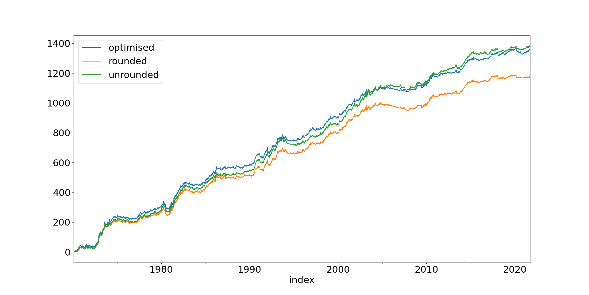
So if we were able to take fractional positions (which we're not!) we could make the green line (which has a Sharpe Ratio of 1.17). But we can't take fractional positions! (sad face and a Sharpe Ratio of just 1.06). But if we run the optimiser, we can achieve the blue line, even without requiring fractional positions. Which has a Sharpe Ratio of .... drumroll... 1.19.
Costs? About 0.13 SR units for all three versions.
Tiny differences in Sharpe Ratio aside, the optimisation process does a great job in getting pretty close to the raw unrounded portfolio (correlation of returns 0.94). OK the rounded portfolio is even more correlated (0.97) , but I think that's a price worth paying.
That's a little higher than what you will have seen in previous backtests. The reason is I'm now including holding costs in my calculations. I plan to exclude some instruments from trading whose holding costs are a little high, which will bring these figures down, but for now I've left them in.
If I do a t-test comparing the returns of the three account curves I find that the optimised version is indistinguishable from the unrounded fractional position version. And I also find that the optimised version is significantly better than the rounded positions: a T-statistic of 3.7 with a tiny p-value. Since these are the versions we can actually run in practice, that is a stonking win for the optimisation.
Risk
The interesting thing about the greedy algorithm is that it gradually adds risk until it finds the optimal position, whilst trying to reduce the variance of the delta portfolio, so it should hopefully target similar risk. Here is the expected (ex-ante) risk for all three systems:
 |
Red line: original system with rounded positions, Green line: original system with unrounded positions, Blue line: optimised system with unrounded positions |
It's quite hard to see what's going on there, so let's zoom into more recent data:

You can see that the optimiser does a superb job of targeting the required risk, compared to the systematically under-risked (in this period - sometimes it will be over-risked) and lumpy risk presented by the rounded positions. The ex-post risk over the entire dataset comes in at 22.4% (unrounded), 20.9% (rounded) and 21.6% (optimised); versus a target of 20%.
How many positions do we typically take?
An interesting question that Doug asked me is how many positions the optimiser typically takes.
"Curious how many positions it uses of the 45??
I guess I don’t know how much capital you are running, but given there are really only maybe 10 independent bets there (or not many more) does it find a parsimonious answer that you might use even if you had a giant portfolio to run?"
Remember we have 45 markets we could choose from in this setup, how many do we actually use?
 |
| Blue line: Total number of instruments with data. Orange line: Instruments with positions from optimiser |
"Pretty cool. The dimension of the returns just isn’t all that high even though there are so many things moving around."
Interestingly, here are some statistics showing the % of time any given instrument has a position on. I've done this over the last 7 years, as otherwise it would be biased towards instruments for which we have far more data:
PALLAD 0.00
COPPER 0.00
GASOILINE 0.00
FEEDCOW 0.00
PLAT 0.00
HEATOIL 0.00
GBP 0.01
REDWHEAT 0.02
WHEAT 0.02
EUR 0.02
NZD 0.03
CRUDE_W_mini 0.03
US20 0.03
US10 0.03
SOYOIL 0.04
LEANHOG 0.04
AUD 0.04
LIVECOW 0.05
JPY 0.05
SOYMEAL 0.06
CAC 0.07
SOYBEAN 0.08
OATIES 0.08
OAT 0.09
RICE 0.10
US5 0.11
MXP 0.12
CORN 0.13
BTP 0.14
SMI 0.14
AEX 0.14
GOLD_micro 0.19
EUROSTX 0.23
KR10 0.24
BITCOIN 0.26
EU-DIV30 0.33
BUND 0.39
EDOLLAR 0.39
BOBL 0.43
NASDAQ_micro 0.47
VIX 0.55
SP500_micro 0.60
KR3 0.66
US2 0.73
SHATZ 0.74
Notice we end up taking positions in all but six instruments. And even if we never take a position in those instruments, their signals are still contributing to the information we have about other markets. Remember from the previous posts, I may want to include instruments in the optimisation that are too illiquid or expensive to trade, and then subsequently not take positions in them.
I've highlighted in bold the 16 instruments we trade the most. You might want to take the approach of only trading these instruments: effectively ignoring the dynamic nature of the optimisation and saying 'This is a portfolio that mostly reproduces the exposure I want'.
However notice that they're all financial instruments (Gold and Bitcoin, quasi financial), reflecting that the big trends of the last 7 years have all been financial. So we'd probably want to go further back. Here are the instruments with the most positions over all the data:
PLAT 0.24
RICE 0.25
CRUDE_W_mini 0.26
NASDAQ_micro 0.27
SOYMEAL 0.33
US2 0.35
US5 0.38
WHEAT 0.39
LIVECOW 0.40
LEANHOG 0.41
CORN 0.43
SOYOIL 0.44
EDOLLAR 0.46
SP500_micro 0.56
GOLD_micro 0.56
OATIES 0.61
That's a much more diversified set of instruments. But I still don't think this is the way forward.
Tracking error
Tracking error: I like to think of as quantified regret. Regret that you're missing out on trends in markets you don't have a full size position in...
What does the tracking error look like? Here are the differences in daily returns between the unrounded and optimised portfolio:

The standard deviation is 0.486%. It also looks like the tracking error has grown a little over time, but 2020 aside it has been fairly steady for a number of years. My hunch is that as we get more markets in the dataset it becomes more likely that we'll have fractional positions in a lot of markets that the optimiser can't match very well. And indeed, if I plot the tracking error of rounded versus unrounded portfolios, it shows a similar pattern. The standard deviation for that tracking error is also virtually identical: 0.494%.
Checking the cost effects
It's worth checking to see what effect the cost penalty is having. I had a quick look at Eurodollar, since we know from the above analysis that it's a market we normally have a position on. Zooming in to recent history to make things clearer:

The green line is the unrounded position we'd ideally want to have on, wheras the red line shows our simple rounded (and buffered) position. The blue line shows what the optimiser would do without a cost penalty. It trades - a lot! And the orange line shows our optimised position. It's trading a bit more than the red line, and interestingly often has a larger position on (where it's probably taking on more of the load of being long fixed income from other instruments), but it's definitely trading a lot less than the blue line.
Interestingly the addition of the cost penalty doesn't reduce backtested costs much, and reduces net performance a little: about 1 SR point, but I'd still rather have the penalty thanks very much.
Much lower capital
To ssee how robust this approach is, let's repeat some of the analysis above with just 50K in capital.

So the optimised version is still better than the rounded (SR improvement around 0.1), but nowhere near as good as the unrounded (SR penalty around 0.2). We can't work miracles! With 50K we just don't have enough capital to accurately reflect the exposures we'd like to take in 45 markets. The tracking error vs the unrounded portfolio is 0.72% for the optimiser (versus 0.49% earlier with 100K), but is even higher for the rounded portfolio (0.76%). The correlation between the optimiser and ideal unrounded optimal returns has dropped to 0.86 (0.94 with 100K); but for rounded positions is even lower: 0.84 (0.97 with 100K).
Less capital makes it harder to match the unrounded position of a large portfolio of instruments, but relatively speaking the dynamic optimisation is still the superior method.
Important note: With
What does this mean?
Let's just review what our options are if we have limited capital, of say $100K:
- We could win the lottery and trade the unrounded positions.
- We could try and trade a lot of instruments - say 45 - and just let our positions be rounded. This gives us a SR penalty of around 0.1 SR versus what we could do with unrounded positions. The penalty would be larger (in expectation) with less capital and / or more instruments (eg it's 0.3SR with 50k). The tracking error would also get larger for smaller capital, relative to the number of instruments.
- We could try and choose a set of static instruments and just trade those. In this post I showed that we could probably choose 16 instruments using a systematic approach. This would also give us a SR penalty of around 0.1 SR in expectation, but the tracking error would be larger than for rounded positions. Again with less capital / more instruments both penalties and tracking error would be larger.
- We could use the 'principal components' approach, to choose a static list of the 16 instruments that are normally selected by the optimiser. I've highlighted these in the list of instruments above. Our tracking error would be a little smaller (in expectation) than for rounded positions, but we'd still have a SR penalty of around 0.1 SR.
- We could have as many instruments as we liked in our portfolio and use the dynamic optimisation approach to decide which of those to hold positions for today. Normally this means we'll only have positions in around 10 instruments or so, but the 10 involved will change from day to day. Our tracking error would be similar as for rounded positions, but we'd not be giving up much in terms of SR (if anything). With smaller capital or more instruments we'd get some SR penalty (but less than the alternatives), and higher tracking error (but again better than the alternatives).
Ignoring the first option, it strikes me that dynamic optimisation brings significant benefits, which for me overcome the additional complexity it introduces into our trading.
Live trading
If you're clever, you will have noticed that the algo code above doesn't include any provision for some of the features I specified in my initital post on this subject:
- A 'reduce only' constraint, so I can gradually remove instruments which no longer meet liquidity and cost requirements
- A 'do not trade' constraint, if for some reason
- Maximum position constraints (which could be for any reason really)
The psystemtrade version of the code here covers these possibilities. It adjusts the starting weights and direction depending on the constraints above, and also introduces minima and maxima into the optimisation (and prevents the greedy algorithim from adjusting weights any further once they've hit those). It's a bit complicated because there are quite a few corner cases to deal with, but hopefully it makes sense.
Note: I could use a more exhaustive grid search for live trading, which only optimises once a day, but I wouldn't be able to backtest it with 100+ instruments so I'll stick with the greedy algorithim, which also has the virtue of being a very robust and stable process and avoids duplicating code.
Let's have a play with this code and see how well it works. Here's what the optimised positions are for a particular day in the data. In the first column is the portfolio weight per contract. The previous days portfolio weights are shown in the next column. The third column shows the optimal portfolio weights we'd have in the absence of rounding. The optimised positions are in the final column. I've sorted by optimal position, and removed some very small weights for clarity:
              per contract  previous  optimal  optimised
SHATZ                 1.32    -10.56    -3.08      -5.27
BOBL                  1.59     -1.59    -1.09       0.00
OAT                   1.97      0.00    -0.31       0.00
VIX                   0.24      0.00    -0.14      -0.24
EUR                   1.47      0.00    -0.13       0.00... snip...
GOLD_micro            0.18      0.00    -0.01      -0.18
... snip...

AEX                   1.84      1.86     0.12       0.00
EUROSTX               0.48      0.00     0.13       0.48
EU-DIV30              0.22      0.22     0.14       0.00
MXP                   0.25      0.00     0.16       0.00
US10                  1.33      1.33     0.17       1.33
SMI                   1.27      0.00     0.19       0.00
SP500_micro           0.22      0.00     0.21       0.00
US20                  1.64      0.00     0.23       0.00
NASDAQ_micro          0.30      0.31     0.26       0.30
US5                   1.23      2.47     0.33       2.47
KR10                  1.07      0.00     0.41       0.00
BUND                  2.01      0.00     0.91       0.00
EDOLLAR               2.47      0.00     1.44       0.00
KR3                   0.94      3.77     2.96       3.77
US2                   2.20      8.81    17.44       8.81
Now let's suppose we could only take a single contract position in US 5 year bonds, which is a maximum portfolio weight of 1.23:
              weight per contract  previous  optimal  optimised  with no trade
SHATZ                        1.32    -10.56    -3.08      -5.27          -2.63
BOBL                         1.59     -1.59    -1.09       0.00           0.00
OAT                          1.97      0.00    -0.31       0.00           0.00
VIX                          0.24      0.00    -0.14      -0.24          -0.24
... snip...GOLD_micro                   0.18      0.00    -0.01      -0.18           0.00
... snip...AEX                          1.84      1.86     0.12       0.00           0.00
EUROSTX                      0.48      0.00     0.13       0.48           0.48
EU-DIV30                     0.22      0.22     0.14       0.00           0.00
MXP                          0.25      0.00     0.16       0.00           0.00
US10                         1.33      1.33     0.17       1.33           1.33
SMI                          1.27      0.00     0.19       0.00           0.00
SP500_micro                  0.22      0.00     0.21       0.00           0.00
US20                         1.64      0.00     0.23       0.00           0.00
NASDAQ_micro                 0.30      0.31     0.26       0.30           0.30
US5                          1.23      2.47     0.33       2.47           1.23
KR10                         1.07      0.00     0.41       0.00           0.00
BUND                         2.01      0.00     0.91       0.00           0.00
EDOLLAR                      2.47      0.00     1.44       0.00           0.00
KR3                          0.94      3.77     2.96       3.77           3.77
US2                          2.20      8.81    17.44       8.81           8.81
That works. Notice that to compensate we reduce our short in two correlated market (German 2 year bonds and Gold, both of which have correlations above 0.55); for some reason this is a better option that increasing our long position elsewhere.
Now suppose we can't currently trade German 5 year bonds, Bobls, (but we remove the position constraint):
              weight per contract  previous  optimal  optimised  with no trade
SHATZ                        1.32    -10.56    -3.08      -5.27          -2.63
BOBL                         1.59     -1.59    -1.09       0.00          -1.59
OAT                          1.97      0.00    -0.31       0.00           0.00
VIX                          0.24      0.00    -0.14      -0.24          -0.24
... snip...GOLD_micro                   0.18      0.00    -0.01      -0.18          -0.18
... snip ...AEX                          1.84      1.86     0.12       0.00           0.00
EUROSTX                      0.48      0.00     0.13       0.48           0.48
EU-DIV30                     0.22      0.22     0.14       0.00           0.00
MXP                          0.25      0.00     0.16       0.00           0.00
US10                         1.33      1.33     0.17       1.33           2.66
SMI                          1.27      0.00     0.19       0.00           0.00
SP500_micro                  0.22      0.00     0.21       0.00           0.00
US20                         1.64      0.00     0.23       0.00           0.00
NASDAQ_micro                 0.30      0.31     0.26       0.30           0.30
US5                          1.23      2.47     0.33       2.47           1.23
KR10                         1.07      0.00     0.41       0.00           0.00
BUND                         2.01      0.00     0.91       0.00           0.00
EDOLLAR                      2.47      0.00     1.44       0.00           0.00
KR3                          0.94      3.77     2.96       3.77           3.77
US2                          2.20      8.81    17.44       8.81           8.81
Our position in Bobl remains the same, and to compensate for the extra short we go less short 2 year Shatz, longer 10 year German bonds (Bunds), and there is also some action in US 5 year and 10 year bonds.
Finally consider a case when we can only reduce our position. There are a limited number of markets where this will do anything in this example, so let's do it with Gold and Eurostoxx (which the previous day have zero position, so this will be equivalent to not trading)
                weight per contract  previous  optimal  optimised  reduce only
SHATZ                        1.32    -10.56    -3.08      -5.27        -5.27
BOBL                         1.59     -1.59    -1.09       0.00         0.00
OAT                          1.97      0.00    -0.31       0.00         0.00
VIX                          0.24      0.00    -0.14      -0.24        -0.24
EUR                          1.47      0.00    -0.13       0.00         0.00
... snip ...GOLD_micro                   0.18      0.00    -0.01      -0.18         0.00
... snip ...EUROSTX                      0.48      0.00     0.13       0.48         0.00
EU-DIV30                     0.22      0.22     0.14       0.00         0.22
MXP                          0.25      0.00     0.16       0.00         0.00
US10                         1.33      1.33     0.17       1.33         1.33
SMI                          1.27      0.00     0.19       0.00         0.00
SP500_micro                  0.22      0.00     0.21       0.00         0.22
US20                         1.64      0.00     0.23       0.00         0.00
NASDAQ_micro                 0.30      0.31     0.26       0.30         0.30
US5                          1.23      2.47     0.33       2.47         1.23
KR10                         1.07      0.00     0.41       0.00         0.00
BUND                         2.01      0.00     0.91       0.00         0.00
EDOLLAR                      2.47      0.00     1.44       0.00         0.00
KR3                          0.94      3.77     2.96       3.77         3.77
US2                          2.20      8.81    17.44       8.81         8.81
Once again the exposure we can't take in Eurostoxx is pushed elsewhere: into EU-DIV30 (another European equity index) and S&P 500; the fact we can't go as short in Gold is compensated for by a slightly smaller long in US5 year bonds.
What's next
I've prodded and poked this methodology in backtesting, and I'm fairly confident it's working well and does what I expect it to. The next step is to write an order generation layer (the bit of code that basically takes optimal positions and current live positions, and issues orders: that will replace the current layer, which just does buffering), and develop some additional diagnostic reports for live trading (the sort of dataframes in the section above would work well, to get a feel for how maxima and minima are affecting the results). I'll then create a paper trading system which will include the 100+ instruments I currently have data for.
At some point I'll be ready to switch my live trading to this new system. The nice thing about the methodology is that it will gradually transition out of whatever positions I happen to have on into the optimal positions, so there won't be a 'cliff edge' effect of changing systems (I might impose a temporarily higher shadow cost to make this process even smoother).
In the mean time, if anyone has any ideas for further diagnostics that I can run to test this idea out I'd be happy to hear them.
Finally I'd like to thank Doug once again for his valuable insight.
very cool, so effectively your are reweighting the portfolio based on their covariance of returns, and if we do this frequently enough (say daily) instruments will gradually get weighted in or out of the portfolio.
ReplyDeleteHow does this new optimization affect your findings regarding diversification vs. maximum number of contracts, as described in https://qoppac.blogspot.com/2016/03/diversification-and-small-account-size.html , notably the "Putting it together" section?
ReplyDeleteIt kind of side steps the problems described in that post by taking a different approach - those findings are still valid.
DeleteHi Rob, how do you run the optimized backtest?
ReplyDeletehttps://gist.github.com/robcarver17/11ec3a6c4370aa8e10c895a483420650
DeleteThanks Rob!
DeleteMissing some files under private folder:
ReplyDelete---> 12 from private.systems.carrytrend.rawdata import myFuturesRawData
... ...
ModuleNotFoundError: No module named 'private.systems'
Not sure if you saw my subsequent comment but I was not able to run the above script as it was referencing a missing file: private.systems.carrytrend.rawdata. Is this something that you can share too?
ReplyDeleteOh you don't need that, the normal rawdata does just fine. I've updated the gist accordingly.
DeleteI ran the backtest and got the below stats using the latest market data downloaded from github:
Delete[[('min', '-9290'),
('max', '9770'),
('median', '35.34'),
('mean', '73.9'),
('std', '1284'),
('skew', '-0.01053'),
('ann_mean', '1.892e+04'),
('ann_std', '2.054e+04'),
('sharpe', '0.9212'),
('sortino', '1.282'),
('avg_drawdown', '-1.693e+04'),
('time_in_drawdown', '0.9387'),
('calmar', '0.2471'),
('avg_return_to_drawdown', '1.117'),
('avg_loss', '-853.1'),
('avg_gain', '939.2'),
('gaintolossratio', '1.101'),
('profitfactor', '1.179'),
('hitrate', '0.5172'),
('t_stat', '6.685'),
('p_value', '2.405e-11')],
('You can also plot / print:',
['rolling_ann_std', 'drawdown', 'curve', 'percent'])]
You can see the equity curve here:
https://ibb.co/qCpsNv5
and it looked different from the one you posted above for recent years. Can you check my results and see if they look ok to you?
That's weird: I just checked with both database and .csv data and didn't get that at all. Exactly what command did you run after the script to get the account curve results?
DeleteIt must be something that I did wrongly then.
ReplyDeleteI ran these 2 lines after the last line in the script.
system.accounts.portfolio().stats()
system.accounts.portfolio().curve().plot()
Is it possible to run the backtest using the csv files? I might not have correctly imported the data into Mongo.
Ah my fault for poor documentation. Those lines will return you the p*l if you just run with rounded, unoptimised, positions. To get the optimised positions do:
Deletesystem.accounts.optimised_portfolio()
To use csv:
from sysdata.sim.csv_futures_sim_data import csvFuturesSimData
Then within def futures_system_dynamic(), use data = csvFuturesSimData() rather than data = dbFuturesSimData()
Thanks Rob, all good now! How do I run the unrounded, unoptimised backtest?
ReplyDeletesystem.accounts.portfolio(roundpositions=False).stats()
DeleteThank you so much Rob! There is so much info and knowledge here that I need to understand. Really appreciate your sharing!
DeleteHey Rob, how can I get the actual positions now using the optimised portfolio? I used to be able to run get_actual_positions but I think it is not available now under system.optimised_portfolio().
ReplyDeleteHi Rob, not sure if you have seen my earlier question regarding seeing the optimised position for a single instrument. I tried running system.portfolio.get_notional_position('AEX') after system.accounts.optimised_portfolio() but the results looked like unrounded positions. Is that right?
ReplyDeleteYeah cos you need system.optimisedPositions.get_optimised_position_df()['AEX']
DeleteThanks! Still trying to understand your system and codes. It's huge! Btw, what other considerations do you consider when selecting an instrument for trading other than looking at its cost and long-term pnl?
DeleteNO I DO NOT LOOK AT P&L!!!
DeleteSo cost
And liquidity
And diversification, for my normal system
Thanks! Make sense!
DeleteHi Rob, not sure where I should post this but I'm trying to think of a easier way to update the futures csv files without going thru the laborious task of stitching prices from different months. For example, I found the Euro BOBL continuous contract data from marketwatch.com: https://www.marketwatch.com/investing/future/fgbm00/download-data?countrycode=de&iso=xeur&mod=mw_quote_tab
ReplyDeleteIt shows OHLC daily prices. Which price should I pick to update the CSV file? Is it the closing price?
I use closing prices.
DeleteThanks Rob!
DeleteDo you have a Discord channel or forum where I can ask you questions regarding your system?
ReplyDeleteI had to google "Discord", so that hopefully answers that question.
DeleteThis is the forum I'm most active on https://www.elitetrader.com/et/threads/fully-automated-futures-trading.289589/page-296
Great! I will hop onto the elitetrader then.
DeleteAlso, I'm new to futures trading. Can I confirm the following?
BITCOIN => Bitcoin CME Futures
CRUDE_W_mini => E-mini Light Crude Oil Futures
EU-DIV30 => DJ Euro Stoxx Select Dividend 30 Index Futures
EUROSTX => DJ Euro Stoxx 50 Futures
NASDAQ_micro => Micro E-mini Nasdaq-100 Index Futures
OAT => French Govt Bonds Futures (FOAT)
REDWHEAT => KC HRW Wheat Futures
OATIES => Oat Futures
SP500_micro => Micro E-mini S&P 500 Index Futures
RICE => Rough Rice Futures
HEATOIL => NY Heating Oil (Platts) Futures
GASOILINE => RBOB Gasoline Futures
VIX => S&P 500 VIX Futures
https://github.com/robcarver17/pysystemtrade/blob/master/data/futures/csvconfig/instrumentconfig.csv
DeleteThanks! Very helpful. For CRUDE_W, do you always trade the Dec contract? For HEATOIL, is it the one traded on ICE?
DeleteYes. You can see it for everything here:
Deletehttps://github.com/robcarver17/pysystemtrade/blob/master/data/futures/csvconfig/rollconfig.csv
No, NYMEX. Again all are here:
https://github.com/robcarver17/pysystemtrade/blob/master/sysbrokers/IB/ib_config_futures.csv
Awesome! Thank you.
DeleteIf I run the script for the optimized system just for EDOLLAR (i.e. 1 instrument) using VS Code, it will crash after a few mins. Certain other instruments like US20 have the same problem as well. Any idea why?
ReplyDeleteAlso can you explain what dm_max means for the below line?
system.config.instrument_div_mult_estimate['dm_max'] = 5
Why is it value 5? Is this parameter same as the capped forecast +20/-20 as mentioned in your LT book?
On page 294 of your LT book, why did you divide by 2 when calculating the transaction cost for FX?
Optimising for one instrument makes no sense... if you were only trading one instrument the optimal position is the rounded position of that instrument.
DeleteThat's the instrument diversification multiplier (described in both LT and my first book, ST). It makes sure the risk of a portfolio of traded instruments hits your vol target; basically the bigger the number the more diversified your portfolio is, the more you need to scale up your risk.
I had a default maximum of this value of 2.5, but a value closer to 3 is needed with the very large 100+ instrument portfolios I can now test with this method (I set it to 5 as an arbitrary maximum to make sure there was no capping here; but it could equally be 3)
I'd dividing the bid/offer spread by two. The slippage if you can trade at the inside spread is the difference between the mid and the bid or offer; which is half the spread.
Also, what's 'VS' code???
DeleteVS Code is Visual Studio Code, the IDE that I used to run the pysystemtrade
DeleteWhen I ran system.portfolio.get_notional_position("AUD").tail(5), I got some output like this:
ReplyDelete2021-09-30 -0.210896
2021-10-01 -0.208213
2021-10-04 -0.204689
2021-10-05 -0.205964
2021-10-06 -0.208951
Should I multiply -0.208951 * 100000 to get the actual FX position?
All positions are reported in futures contracts.
DeleteSorry, a bit confused, AUD is an FX pair according to instrumentconfig.csv. Why would the position be in futures coontracts?
DeleteBecause I only trade futures.... 'FX' in the configuration means the underlying asset is FX, but it's still a future.
DeleteUnderstood! I've been papertrading the AUD spot using your spreadsheet and I'm thinking of using pysystemtrade to check the results.
DeleteIs there a way to make a config change to report the AUD position as FX and not futures?
Will it be possible to add a new non-futures instrument for AUD Spot in rollconfig.csv, instrumentconfig.csv, ib_config_futures.csv for this purpose?
pysystemtrade is only for futures so I'm reluctant to start adding any non futures instruments, and I also wouldn't want to add anything I don't trade myself. Also the way that position sizing works for FX is completely different than for futures, and depends on what you're trading, so there is much more to this than just changing a single number in a spreadsheet.
DeleteAlso bear in mind that using the AUDUSD future as a proxy to generate a signal for AUD spot involves a huge number of approximations...
No prob, I will use your spreadsheet for FX Spot.
DeleteHi Mr.Rob Carver. My name is Nanthawat Anancharoenpakorn. I read several of your book and I realized that I have a hugh room to learn. May I kindly ask you for some advice :)
ReplyDeleteHere are the situations:
1) I'm 24 year old and going to do Master for leverage my knowledge.
2) study Finace and basic programming
3) My purpose is clear : To be systematic trader. (just like you or similar)
- or To have similar skill set or experience
Here are the questions :
1) Which Master degree faculty is most suitable for systematic trading skill set (any advice for University or faculty)
2) what you would like to tell yourself if you were 24
3) Any advice for those 24 who want to be systematic trader.
4) Any advice about life (would be nice)
*If you already post about this please let me know where to go :)
Thank you!
I'm Really Appreciated
https://qoppac.blogspot.com/2021/02/so-you-want-to-be-quantsystematic-trader.html
DeleteI can't recommend specific courses or unis
This comment has been removed by a blog administrator.
ReplyDeleteRob Ignore previous comment I found it.
ReplyDeleteRory Mackay
Mr. Carver,
ReplyDeletelove your books! I am learning a great deal and I would like to thank you for that!
Trying to wrap my head around dynamic optimization and tracking errors.
The issue of dynamic optimization reminds me of a promising solution by Nick Baltas. It is an equal risk contribution approach that dynamically adapts not only to changing volatilities but also to changing correlations. The strength of the solution becomes clrearly visible in times of rising correlations.
The original paper:
https://deliverypdf.ssrn.com/delivery.php?ID=708020093087023090084074073094096109059004061032064017118121013005088091031084097089101045036122006102119119113116026116002090060018059064034114125004087015069090062048016111072087030019006100115122021121127125084004071064087025080030089088093110098&EXT=pdf&INDEX=TRUE
Neatly summarized as ppt presentation: https://pdfs.semanticscholar.org/c96d/3a49be9b92da6bec20aecb7ed7c10a190fd5.pdf
Using that approach would allow to disregard the less precise instrument diversification multiplier. We could still use forecasts to deduce signal strength but scaling into positions wouldn’t work as the weight is defined by the marginal risk contribution.
Precisely measuring the risk contribution of each asset while factoring in the correlations seems really conveniant. Even more precise would be to measure the MRC of the trading strategy and not the MRC of the underlying asset. We know trading a trend following strategy can change the properties of the distribution of returns compared to the return distribution of the traded asset.
Somebody was nice enough to code all strategies mentioned in the paper and put it on github:
https://github.com/MasterFinHEC/ASSET_PROJECT
As far as I understand the goal of the greedy algo solves a different issue namely the problem of fractional positions.
This approach could still add value, right?
It sounds different than what you have tried but maybe I am missing something.
Timo
I wish I had the time to read and understand the paper but I don't
DeleteEssentially he argues that in the literature of trend following the expression “risk parity” is often used for approaches that use vol targeting. “True risk parity” takes the (ever changing) correlations into account and adapts the portfolio accordingly. Risk parity is only defined for long portfolios. Therefore he adapts the formula so it can be traded long and short. Overall very similar to your writings. Merely the way of incorporating the correlations is different to yours though I can’t say whether the results would differ significantly.
Delete(slide 16 on page 17 gives a good overview in case you should ever come back to the question whether another way could push the boundaries of diversification even further…)
I might try it out. In case I do I would be happy to share the backtest results if you think it is worth your time…
Dear Rob, I've just found your blog by random chance and thus spent the day reading it :)
ReplyDeleteIt has been amusing that on December 2024 I got your "Systematic Trading" book and after reading it a couple of times, on January I decided to code essentially a greedy search for the optimal number of contracts based on trying to match a target volatility.
I'm reading it again now and it even has a cute comment that you will be familiar with: "TODO: While rem_delta > 0, remove low volatility and add high volatility."
Anyways, just a note here.. let me subscribe to the RSS and will slowly read all the posts over time ^_^