- How should we control risk (first post)
- How much risk should we take? (previous post)
- How fast should we trade? (this post)
As with the other two posts this topic is covered in much more detail in my two books on trading: "Systematic Trading" and "Leveraged Trading"; although there is plenty of new material in this post as well. If you want more information, then it might be worth investing in one of those books. "Leveraged Trading" is an easier read if you're relatively new to trading.
The timing of my posts about risk has turned out to be perfect, with the Coronavirus currently responsible for severe market movements as well as thousands of deaths. It's less obvious why trading too frequently is a problem. The reason is costs. Taking on too much risk will lead to a fast blowup in your account. Trading too often will result in high costs being paid, which means your account will gradually bleed to zero. As I write this, I notice for the first time how often we use metaphors about losing money which relate to death. For obvious reasons I will try and avoid these for the rest of the post.
Incidentally, I'm not going to post anything about 'trading and investing through the Coronavirus'. I have put a few bits and pieces on twitter, but I don't feel in the mood for writing a long post about exploiting this tragedy for financial gain.
Neithier will I be writing anything about the likely future path of markets from here. As you know, I don't feel that making predictions about price movements is something I'm especially good at. I leave that to my trading systems. Finally, I won't be doing any analysis of the models used for predicting Coronavirus deaths. I leave that to epidemiologists.
I will however be posting my normal annual update on performance after the UK tax year ends in a few days time. And I will probably, at some point in the future, write a post reviewing what has happened. But not yet.
Overview
How fast should we trade? We want to maximise our expected returns after costs. That's the difference between two things:
- Our pre-cost returns
- Our costs
The structure of this post is as follows: Firstly I'll discuss the measurement and forecasting of trading costs. Then I will discuss how expected returns are affected by trading speed. Finally I will talk about the interaction between these two quantities, and how you can use them to decide how quickly to trade.
Types of costs
There are many different kinds of costs involved in trading. However there are two key categories:
- Holding costs
- Trading costs
Holding costs are costs you pay the whole time you have a position on, regardless of whether you are trading it. Examples of holding costs include brokerage account fees, the costs of rolling futures or similar derivatives, interest payments on borrowing to buy shares, funding costs for FX positions, and management fees on ETFs or other funds.
Trading costs are paid every time you trade. Trading costs include brokerage commissions, taxes like UK stamp duty, and the execution costs (which I will define in more detail below).
Some large traders also pay exchange fees, although these are normally included as part of the brokerage commission. Other traders may receive rebates from exchanges if they provide liquidity.
The basic formula for calculating costs then is:
Total cost per year = Holding cost + (Trading cost * Number of trades)
Execution costs
Most types of costs are pretty easy to define and forecast, but execution costs are a little different. Firstly a definition: the execution cost for a trade is the difference between the cost of trading at the mid-price, and the actual price traded at.
So for example if a market is 100 bid, 101 offer, then the mid-price is just the average of those: 100.5
Some people calculate the mid price as a weighted average, using the volume on each side as the weight. Another term for this cost is market impact.
If we do a market order, and our trade is small enough to be met by the volume at the bid and offer, then our execution cost will be exactly half the spread. If our order is too large, then our execution cost will be larger.
 |
| Who actually earns the execution cost you pay? Judging by his smile, it's this guy |
Broadly speaking, we can estimate execution costs or measure them from actual trading. You can estimate costs by looking at the spreads in the markets you trade, or using someone elses estimates.
A nice paper with estimates for larger traders is this paper by Frazzini et al, check out figure 4. You can see that someone trading 0.1% of the market volume in a day will pay about 5bp (0.05%) in execution costs. Someone trading 0.2% of the volume will pay 50% more, 7.5bp (0.075%).
When estimating costs, there are a few factors you need to bear in mind. Firstly, the kind of trading you are doing. Secondly, the size of trading.
- Smaller traders using market orders: Assume you pay half the spread
- Smaller traders using limit orders or execution algos: You can pay less, but (I pay about a quarter of the spread on average, using a simple execution algo)
- Larger traders: Will pay more than half the spread, and will need to acccount for their trading volume.
You can use execution algos (which mix limit and market orders) if you are trading reasonably slowly. You can use limit orders if you're trading a mean reversion type strategy of any speed, with the limits placed around your estimate of fair value (though you may want to implement stop-losses, using market orders). If you are trading a fast trend following strategy, then you're going to have to use market orders.
If you're trading very quickly, then assuming a constant cost of trading is probably unrealistic since the market will react to your order flow and this will significantly change your costs. In this case I'd suggest only using figures from actual trades.
There are other ways to reduce costs, such as smoothing your position or using buffering. If you are trading systematically you can incorporate these into your back-test to see what effect they have on your cost estimates.
Linear and non-linear
An important point here is that smaller traders, to all intents and purposes, face fixed execution costs per trade. If they double the number of trades they do, then their trading costs will also double. Smaller traders have linear trading costs.
Holding costs will be unaffected by trading, and other costs eg commissions may not increase linearly with trade size and frequency, but this is a reasonable approximation to make.
But larger traders face increasing trading costs per trade. If they do larger size or or more trades, their costs per trade will increase (eg from 5bp to 7.5bp in the figures given in the Frazzini paper above). If they double the number of trades they do their execution costs will more than double; using the figures above they will increase be a factor of 3: twice because they are doing double the number of trades, and then by another 50% as the cost per trade is increasing. Larger traders have non linear trading costs.
Normalisation of costs
What units should we measure costs in? Should it be in pips or basis points? Dollars or as a percentage of our acount value?
For many different reasons I think the best way to measure costs is as a return adjusted for risk. Risk is measured, as in previous posts, as the expected annualised standard deviation of returns.
Suppose for example that we are buying and selling 100 block shares priced at $100 each. The value of each trade is $10,000. We work out our trading costs at $10 per trade, which is 0.1%. The shares have a standard deviation of 20% a year. So each trade will cost us 0.1 / 20 = 0.005 units of risk adjusted return. Notice how similar this is to the usual measure of risk adjusted returns, the Sharpe Ratio. We are effectively measuring costs as a negative Sharpe Ratio.
We don't include a risk free rate in this calculation, as otherwise we'd end up cancelling it out when we subtract costs as a Sharpe Ratio from pre-cost returns measured in the same units.
Why does this make sense? Well, it makes it easier to compare trading costs across different instruments, account sizes, and time periods. Trading costs measured in dollar terms look very high for a large futures contract like the S&P 500, but they're actually quite low. Because of the COVID-19 crisis, spreads in most markets are pretty wide at the moment, but this means costs in risk adjusted terms are actually pretty similar.
It also relates to how we scale positions in the second post of this series. Since we scale positions according to the risk of an instrument, it makes sense to scale costs accordingly.
Estimating the number of trades
Let's return to the basic formula above:
Total cost per year = Holding cost + (Trading cost * Number of trades)
We're going to need to calculate the expected number of trades. How to do this?
- We can infer it from the size of our stop-loss relative to volatility, defined in the first post as X (this works no matter what kind of trader you are)
- Systematic Traders: We can get it from a backtest
- Systematic Traders: We can use some heuristics based on the kind of trading system we are running
You can find heuristics for different trading systems in both of my books on trading; in this post I'm going to focus on the stop loss method as it's simpler, applies to all traders, and is consistent with the methodology I'm using in the other posts.
Here's the table you need:
Fraction of volatility 'X' Average trades per year
0.025 97.5
0.05 76.5
0.1 46.9
0.2 21.4
0.3 11.9
0.4 7.8
0.5 5.4
0.6 4.0
0.7 3.10.8 2.4
0.9 2.1
1.0 1.7
We will use the data in this table later when we try and work out how fast we should be trading.
Trading cost calculations: example
We know have enough information to work out how the trading costs for a given instrument and stop loss fraction.
In my book, "Leveraged Trading", I include examples for all the main types of traded instruments (futures, spot FX, spread bets, CFDs and stock/ETF trading). Here however there isn't really enough space, so I'm just going to focus on my favourite: futures.
As I started out life as a fixed income trader, let's consider the costs of the Eurodollar future. Eurodollars are relatively pricey to trade for a future, but still cheaper than the products most retail investors prefer like CFDs, spread bets and spot FX.
Each contract index point is worth $2500 and the current price of the June 2023 I hold is $99.45 (but that may change!). So each contract has a current notional value of 2500*99.45 = $248,625. My broker charges $1 per contract in commission, and the spread is 0.005 of a point wide (except on the front contract: but don't trade that!).
To trade one contract as a small trader with a market order will cost half of the spread: 0.5*0.005*$2500 = $6.25 plus the commission of a $1 = $7.25. That is 0.0029% of the notional value. There are no taxes or further fees due. It doesn't matter how many contracts we trade, it will always cost 0.0029% of the notional value per trade.
What about holding costs? Each contract has to be rolled quarterly. It's usually possible to do the roll as a calendar spread rather than two seperate trades. This reduces risk, but also means it will cost the same as a regular trade in execution cost (though we will pay two lots of commission). So each roll trade will cost $6.25 plus $2 = $8.25, or 0.00332% of the notional value. Four lots of that per year adds up to 0.0132% in holding costs.
Let's convert these into risk adjusted terms. The risk of Eurodollars is currently elevated, but in more normal times it averages about 0.5% a year. So the execution cost will be 0.0029/0.5 = 0.0058 and the holding cost is 0.0132/0.5 = 0.026. Both in units of Sharpe Ratio.
Here's our formula again:
Total cost per year = Holding cost + (Trading cost * Number of trades)
Total cost per year = 0.026 + (0.0058 * Number of trades)
Total cost per year = 0.026 + (0.0058 *5.4) = 0.058
Pre-cost returns: Theory
Let us now turn our attention to pre-cost returns. How are these affected by trading speed? Naively, if we double the number of trades we do in a given timeframe, can we double our profits?
We can't double our profits, but they should increase. Theoretically if we double the number of trades we do we will increase our profits by the square root of 2: 1.414 and so on. This is down to something called The Law Of Active Management. This states that your 'information ratio' will be proportional to the square root of the number of uncorrelated bets that you make. If we make some assumptions then we can boil this down to your return (or Sharpe Ratio) being proportional to the square root of the number of trades you make in a given time frame.
Pre-cost returns: Practice
LAM is a theory, and effectively represents an upper bound on what is possible. In practice it's extremely unlikely that LAM will always hold. Take for example, the Sage of Omaha.
 |
| Ladies and Gentlemen, I give you Mr Warren Buffet. |
His information ratio is around 0.7 (which is exceptionally good for a long term buy and hold investor), and his average holding period is... well a long time but let's say it's around 5 years. Now under the Law of Active Management what will Warren's IR be if he shortens his holding period and trades more?
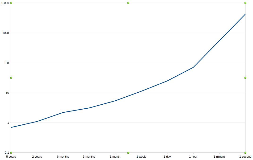 |
| X-Axis: Holding Period. Y-Axis: Information ratio |
Shortening it to 2 years pushes it up to just over 1.0; pretty good and probably achievable. Then things get silly and we need a log scale to show what's going on. By the time Warren is down to a one week holding period his IR of over 10 put's him amongst the best high frequency trading firms on the planet, despite holding positions for much longer.
When the graph finishes with a holding period of one second, still well short of HFT territory, Warren has a four figure IR. Nice, but very unlikely.
This is a silly example, so let's take a more realistic (and relevant) one. The average Sharpe Ratio (SR) for an arbitrary instrument achieved by the slowest moving average crossover rule I use, MAV 64,256, is around 0.28. It does 1.1 trades per year. What if I speed it up by using shorter moving averages, MAV 32,128 and so on? What does the LAM say will happen to my SR, and what actually happens.
 |
| X-axis: Moving average rule N,4N. Y-axis Sharpe Ratio pre-costs |
If I turn the dial all the way and start trading a MAC 2,8 (far left off the graph) the LAM says the Sharpe should be a stonking 1.68. The reality is a very poor 0.07. Momentum just doesn't work so well at shorter timeframes, although it does consistently well between MAC8 and MAC64. You can't just increase the speed of a trading rule and expect to make more money; indeed you may well make less.
Net returns
We are now finally ready to put pre-cost returns together with costs and see what they can tell us about optimal trading speeds. For now, I will stick with using a set of moving average rules and the costs of trading Eurodollar futures. Later in the post I'll discuss how you can set stop-losses correctly in the presence of trading costs.
Let's take the graph above, but now subtract the costs of trading Eurodollar futures using the formula from earlier:
Total cost per year = 0.026 + (0.0058 * Number of trades)
 |
| X-Axis: Moving average rule, Y-axis Sharpe Ratio before and after costs |
The faster rules look even worse now and actually lose money. For this particular trading rule the question of how fast we can trade is clear: as slow as possible. I recommend keeping at least 3 variations of moving average in your system for adequate diversification, but the fastest two variations are clearly a waste of money.
Important: I am comparing the average SR pre-cost across all instruments with the costs just for Eurodollar. I am not using the backtested Sharpe Ratios for Eurodollar by itself, which as it happens are much higher than the average due to secular trends in interest rates. This avoids overfitting.
These results are valid for smaller traders with linear costs. Just for fun, let's apply an institutional level of non linear costs. We assume that costs per trade increase by 50% when trading volume is doubled:
 |
| X-Axis: Moving average rule, Y-axis Sharpe Ratio with LAM holding before and after costs for larger traders |
I'm only showing the LAM here; the actual figures are much worse. Even if we assume that LAM is possible (which it isn't!), then speeding up will stop working at some point (here it's at around MAC16). This is because pre-cost returns are improving with square root of frequency, but costs are increasing more than linearly.
Net returns when returns are uncertain
So far I've treated pre-cost returns and costs as equally predictable. But this isn't the case. Pre-cost returns are actually very hard to predict for a number of reasons. Regular readers will know that I live to quantify this issue by looking at the amount of statistical variation in my estimates of Sharpe Ratio or returns.
Let's look at the SR for the various speeds of trading rules, but this time add some confidence intervals. We won't use the normal 95% interval, but instead I'll use 60%. That means I can be 20% confident that the SR estimate is above the lower confidence line. I also assume we have 20 years of data to estimate the SR:
 |
| X-axis: Moving average variations. Y-axis: Actual Sharpe Ratio pre-costs, with 60% confidence bounds applied |
Notice that although the faster crossovers are kind of rubbish, the confidence intervals still overlap fairly heavily, so we can't actually be sure that they are rubbish.
Now let's add costs. We can treat these as perfectly forecastable with zero sampling variance, and compared to returns they certainly are:
 | |
|
A rule of thumb
All of the above stuff is interesting in the abstract, but it's clearly going to be quite a lot of work to apply it in practice. Don't panic. I have a heuristic; I call it my speed limit:
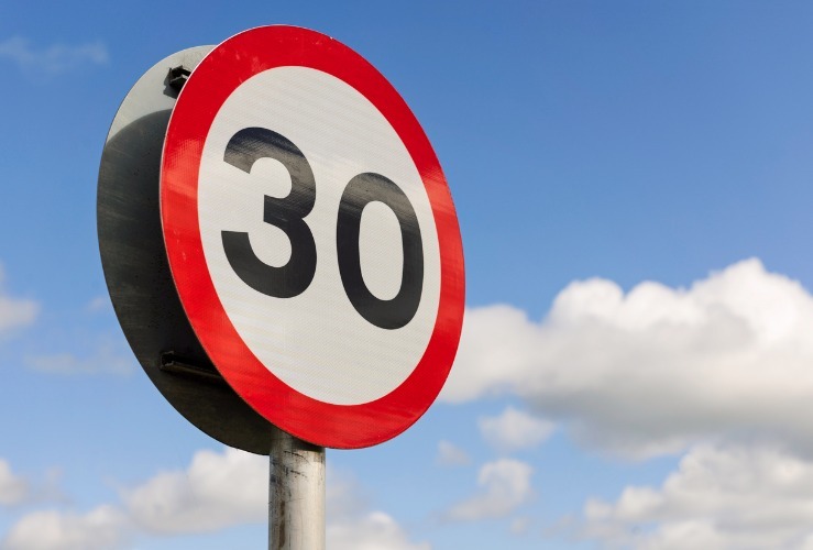
SPEED LIMIT: DO NOT SPEND MORE THAN ONE THIRD OF YOUR EXPECTED PRE-COST RETURNS ON COSTS
How can we use this in practice? Let's rearrange:
Total cost per year = Holding cost + (Trading cost * Number of trades)
(speed limit) Max cost per year = Expected SR / 3
Expected SR / 3 = Holding cost + (Trading cost * Max number of trades)
Max number of trades = [(Expected SR / 3) - Holding cost] / Trading cost
(speed limit) Max cost per year = Expected SR / 3
Expected SR / 3 = Holding cost + (Trading cost * Max number of trades)
Max number of trades = [(Expected SR / 3) - Holding cost] / Trading cost
Specifically for Eurodollar:
Total cost per year = 0.026 + (0.0058 * Number of trades)
Max number of trades = [(Expected SR / 3) - 0.026] / 0.0058
The expected SR varies for different trading rules, but if I plug it into the above formula I get the red line in the plot below:
Total cost per year = 0.026 + (0.0058 * Number of trades)
Max number of trades = [(Expected SR / 3) - 0.026] / 0.0058
The expected SR varies for different trading rules, but if I plug it into the above formula I get the red line in the plot below:
 |
| X axis: Trading rule variation. Y-axis: Blue line: Actual trades per year, Red line: Maximum possible trades per year under speed limit |
The blue line shows the actual trades per year. When the blue line is above the red we are breaking the speed limit. Our budget for trading costs and thus trades per year is being exceeded, given the expected SR. Notice that for the very fastest rule the speed limit is actually negative; this is because holding costs alone are more than a third of the expected SR for MAC2.
Using this heuristic we'd abandon the two fastest variations; whilst MAC8 just sneaks in under the wire. This gives us identical results to the more complicated analysis above.
Closing the circle: what value of X should I use?!
The speed limit heuristic is awfully useful for systematic traders who can accurately measure their expected number of trades and . But what about traders who are using a trading strategy that they can't or won't backtest? All is not lost! If you're using the stoploss method I recommended in the first post of this series, then you can use the table I included earlier to imply what value of X you should have, based on how often you can trade given the speed limit.
For trading a single instrument I would recommend using a value for expected Sharpe Ratio of around 0.24 (roughly in line with the slower MAC rules).
Max number of trades = [(Expected SR / 3) - Holding cost] / Trading cost
Max number of trades = [0.08 - Holding cost] / Trading cost
Let's look at an example for Eurodollars:
Max number of trades = [0.08 - 0.026] / 0.0058 = 9.3
Max number of trades = [0.08 - Holding cost] / Trading cost
Let's look at an example for Eurodollars:
Max number of trades = [0.08 - 0.026] / 0.0058 = 9.3
From the table above:
Fraction of volatility 'X' Average trades per year
... ...
0.3 11.9
0.3 11.9
0.4 7.8
0.5 5.4
... ...
... ...
This implies that the maximum value for 'X' in our stop loss is somewhere between 0.3 and 0.4; I suggest using 0.4 to be conservative. That equates to 7.8 trades a year, with a holding period of about 6 to 7 weeks.
Summary
I've gone through a lot in the last few posts, so let's quickly summarise what you now know how to do:
- The correct way to control risk using stop losses: trailing stops as a fraction of annualised volatility ('X')
- How to calculate the correct position size using current volatility, expected performance, account size, strength of forecast and number of positions.
- The correct value of 'X' given your trading costs
Knowing all this won't guarantee you will be a profitable trader, but it will make it much more likely that you won't lose money doing something stupid!
Do you plan to post the rules for calculating X using ATR?
ReplyDeleteYou can go from ATR to standard deviations, which you would then use to decide the size of your stop loss gap (X*annual_standard_Deviation) From the second post in this series https://qoppac.blogspot.com/2020/03/how-much-risk-should-we-take.html "If you prefer to measure risk using the well known ATR, then as a rule of thumb multiplying the daily ATR by 14 will give you the annual standard deviation."
ReplyDeleteHi Rob,
ReplyDeleteLeveraged Trading (Formula 8) uses 'natural instrument risk'. From the book:
Formula 8: Risk-adjusted transaction costs
Risk-adjusted cost per transaction = Cost per transaction ÷ natural instrument risk
The example then uses a target portfolio risk of 20% as 'natural instrument risk'. What exactly is natural instrument risk?
The annualised standard deviation of returns of the instrument.
DeleteThank you for the clarification. I am implementing your formulas and concepts in C#, hence my desire for accuracy.
DeleteI very much appreciate your efforts in sharing your knowledge through books and this blog. You provide a much needed guide on incorporating risk and cost management into trading.
This comment has been removed by the author.
ReplyDeleteRob,
ReplyDeleteThank you for posting all this, very interesting once again.
I'd like your opinion on different cases that could impact the model.
Just trying to assess if those are worth spending time on.
It will be easier with an example and assuming holding costs = 0.
For example on SP500, I see in your config a slippage of 0.125 and let's assume the SP500 std dev is 16%.
1. Historical half-spreads
The 0.125 half spread corresponds to a snapshot of the current market liquidity. If i understand correctly, if SP500 std dev was also 16% back in 1990 (for example), that implies we would assume the half spread to also be 0.125 in 1990 in the backtest. I do not have access to bid-ask data but I'd imagine that spreads were wider then. What is your opinion on this? What do you think about adding a penalty (maybe in %) that increases the further we go back in time?
2. Lower volatility
Let's assume SP500 vol was 8% at some point in the past (so half the volatility we used when computing the SR costs), the model would imply the half-spread to be 0.125 / 2. But this is not technically possible as the minimum tick size on SP500 is 0.25 so the half-spread could never be less than 0.125. Also, I believe on some futures the current minimum tick size is a fraction of what it was before electronic markets were introduced. Do you think it would make sense to introduce a floor in costs equivalent to that minimum tick size?
3. Higher volatility
The model assumes slippage moves linearly with volatility. With the most recent increase of volatility, is your live execution in line with this assumption?
I know from experience that for option markets the bid-ask usually increases faster than volatility, often in a quadratic way. Interested to know if you observed futures market as being more stable.
Thank you in advance!
One1Hedge
This comment has been removed by the author.
DeleteThese are all excellent questions.
DeleteAn important general point here is that for the sort of trading I am doing getting cost assumptions wrong even by a factor of two has limited effect on my p&l, and almost no effect on the decisions I make in deciding how to trade. It's far better to make a simplifying assumption that means I can use decades of historic data for backtesting.
This clearly wouldn't be the case if I was trading faster or in larger size.
1. Yes it's true that markets have got cheaper to trade over time. But many markets were also more volatile in the past, though clearly not all. This makes it difficult to apply a blanket rule like 'everything cost more in the past'. Without access to genuine historical slippage data anything you do will be an approximation.
This does mean you should be careful; suppose for example you find a fast strategy that worked well in the past but is flat over the last decade or so. Well you know that in the past the costs would have been higher, so really after costs it would have lost money historically. Indeed, this is exactly what happens with faster trend following on equity indices.
This suggests using some kind of moving window or exponential mean of returns, although I'd caution that this shouldn't be too short as we will struggle to get any statistically significant results if we start using just a few years for estimation.
2. You could do this, and a market where it would make most sense is something like the short bonds or STIR where there was a long period when vol was extremely low (now over?)
3. I'd say the real experience is something like this; when the markets get a bit more volatile the inside spread doesn't change but the depth gets much worse. For my relatively small trades that means that trading costs probably don't change much as vol goes up, at least to begin with.
When vol gets very high however the spread will increase. This is probably <1% of the time however.
Plotting slippage against vol would then probably come out as quadratic(ish) rather than linear; flat to begin with then going up. However it would be a different fit to an institutional sized trader.
At some point I ought to do an analysis of my costs data which I have been collecting for several years now to see if I can confirm these hunches.
Thanks for the detailed answers, very clear.
DeleteAnother question for you: looking at the pre-cost chart comparing LAM to actual SR, the fastest rules seem to decay compared to longer term ones. Do you think it could also come from the granularity of the data you use? If you were to use 1min data to backtest equivalent rules (by that, i mean rebuilding an ewmac 2 days / 8 days from the 1min data, not 2 minutes / 8 minutes), the long term slow rules wouldn't change much with the extra intraday information but the shorter term faster rules would probably rebalance more often and catch more of the intraday trends. Or maybe another way to look at it, if you restricted the slower rules so they can only trade once a week/month (or whatever the equivalent would be of a daily rebalancing for the fastest rules), do you think it would make the performance uniform?
Thank you
Throttling the slower rules wouldn't affect the performance very much, although it would introduce more dispersion in the outcome (since the exact date of rebalancing can affect the p&l, versus it being effectively continous).
DeleteI also know from past research that using more granular data wouldn't help with the very fast rules. It does seem like the market has more mean reverting behaviour at this frequency. The stylised facts seem to be:
Greater than 1 year: Mean reversion (eg equity valuations)
~1 month to ~1 year: trend following
~1 day to ~1 month: Mean reversion
~minutes to day: Trend following
sub minute: Mean reversion (market making high frequency)
The cut off time periods seem to depend on the asset class, so for example for equity indices the trend following window is narrower than for other asset classes.
That makes sense, thanks. The cut off time periods you mention are in line with results I get when looking at optimal delta rebalancing frequency for option trading. No surprise there but it's good to have confirmation.
DeleteGreat discussion. It sure sounds like there's an application of Fourier analysis in there somewhere.
DeleteRob,
ReplyDeleteI am trying to implement the full system from leveraged trading (having done the simple system for some time). I have 24 etf instruments I trade as cfds. They are from many different asset classes. I have calculated the Account Level Risk as 25% and the IDM as 2.3 which gives an instrument level risk of 57.5%. These are from the tables in the book. My understanding is that all positions will be leveraged until their standard deviation % is above 57.5%. This makes it highly unlikely any position will ever be unleveraged unless I go mad and trade crypto. The problem is this usually makes my whole account leverage such that the margin with IG (20% retail) is right on the maximum account value with the full account value as margin, leaving no margin for error(pun intended).Is this just a symptom of using the system as a retail investor(and you intended leverage of 5 x plus to be the norm at an account level) or have I made an error? I don't intend to use the maximum 5 x leverage but would like to know if I am on the right lines in my understanding. Thanks for your books and help.
What is the natural unlevered risks of the instruments you are trading? I'm surprised you need 5 times leverage to hit 57% risk unless you have a lot of low volatility short duration bond ETFs.
Deleteyes, the issue is 30% in various bond etfs with very low instrument risk. They are many multiples of leverage as a result causing the overall group of etfs to be 5 x leveraged. Without them leverage drops markedly. Is that the answer?
ReplyDeleteYes. I actually address this in my second book, but the best solution is probably to replace the bond ETFs with some higher vol products, eg longer duration.
Deleteok thanks. I have just bought the second book. Perhaps I should have read it before trying to put something together.
DeleteAs a biginer in systematic trading where can I start.
ReplyDeleteHi Rob, thanks for the post, great as always. I'm backtesting your MA crossover rules and I found similar results; the faster crossovers tend to lose money after factoring cost. My question is how do you "slow down" your system? Do you either
ReplyDelete1) Exclude the fast crossovers rule that are above your speed limit from your final forecast for each asset
2) Retain all the rules to get your final forecast, and then use some sort of smoothing to reduce the turnover
Thanks!
Mostly (1), but I also buffering on the final position which reduces turnover.
Delete