You can see what else has been included in pysystemtrade since you last checked, here. If you're not a fan of pysystemtrade, don't worry, you'll probably find the discussion interesting although you'll then have to work out how to implement it yourself.
Naturally your understanding and enjoyment of this post will be enhanced if you've read chapter 12 of my book, though non readers who have followed my blog posts on the subject of optimisation should also be fine.
This post has been modified to reflect the changes made in version 0.10.0
Costs, generally
In this first part of the post I'll discuss in general terms the different ways of dealing with costs. Then I'll show you how to do this in python, with some pretty pictures.
How to treat costs
Ignore costs - use gross returns
This is by far the simplest option. It's even okay to do it if the assets in your portfolio optimisation, whether they be trading rules or instruments, have the same costs. Of course if this isn't the case you'll end up overweighting anything that looks amazing pre-costs, but has very high costs to go with it.
Subtract costs from gross returns: use net returns
This is what most people would do without thinking; it's perhaps the "obvious" solution. However this skips over a fairly fundamental problem, which is this: We know costs with more certainty than we know expected gross returns.
I'm assuming here you've calculated your costs properly and not been overly optimistic.
Take for example my own trading system. It backtests at something like a 20% average return before costs. As it happens I came in just over that last year. But I expect just over two thirds of my annual returns to be somewhere between -5% and +45% (this is a simple confidence interval given a standard deviation of 25%).
Costs however are a different matter. My costs for last year came in at 1.39% versus a backtested 1.5%. I am pretty confident they will be between 1% and 2% most years I trade. Costs of 1.5% don't affect optimisation much, but if your predicted costs were 15% versus a 20% gross return, then it's important you bear in mind your costs have perhaps a 70% chance of being between 14% and 16%, and your gross returns between -5% and 45%. That's a system I personally wouldn't trade.
The next few alternatives involve various ways of dealing with this issue.
Ignore gross returns, just use costs
This is probably the most extreme solution - throw away any information about gross returns and optimise purely on cost data. Expensive assets will get a lower weight than cheap ones.
(Note this should be done in a way that preserves the covariance structure of gross returns; since we still want more diversifying assets to be upweighted. It's also good for optimisation to avoid negative returns. I apply a drag to the returns such that the asset's Sharpe Ratios are equal to the cost difference plus a reasonable average Sharpe)
I quite like this idea. I think it's particularly appealing in the case of allocating instrument weights in a portfolio of trading systems, each trading one instrument. There is little reason to think that one instrument will do better than another.
Nevertheless I can understand why some people might find this a little extreme, and I probably wouldn't use it for allocating forecast weights to trading rule variations. This is particularly the case if you've been following by general advice not to fit trading models in the "design" phase, which means an optimiser needs to be able to underweight a poor model.
Subtract costs from gross returns, and multiply costs by a factor
This is a compromise where we use gross returns, but multiply our costs by a factor (>1) before calculating net costs. A common factor is 2, derived from the common saying "A bird in the hand is worth two in the bush", or in the language of Bayesian financial economics: "A bird which we have in our possession with 100% uncertainty has the same certainty equivalent value as two birds whose ownership and/or existence has a probability of X% (solve for X according to your own personal utility function)".
In other words 1% of extra costs is worth as much as 2% of extra gross returns. This has the advantage of being simple, although it's not obvious what the correct factor is. The correct factor will depend on the sampling distribution of the gross returns, and that's even without getting into the sticky world of uncertainty adjustment for personal utility functions.
Calculate weights using gross returns, and adjust subsequently for cost levels
 |
| I'm 97% sure this is Thomas Bayes. Ex-ante I was 100%, but the image is from Wikipedia after all. |
In table 12 (chapter 4, p.86 print edition) of my book I explain how you can adjust portfolio weights if you know with certainty what the Sharpe ratio difference is between the distribution of returns of the assets in our portfolio (notice this is not as strong as saying we can predict the actual returns). Since we have a pretty good idea what costs are likely to be (so I'm happy to say we can predict their distribution with something close to certainty) it's valid to use the following approach:
- Make a first stab at the portfolio weights using just gross returns. The optimiser (assuming you're using bootstrapping or shrinkage) will automatically incorporate the uncertainty of gross returns into it's work.
- Using the Sharpe Ratio differences of the costs of each asset adjust the weights.
This trick means we can pull in two types of data about which we have differing levels of statistical confidence. It's also simpler than the strictly correct alternative of bootstrapping some weights with only cost data, and then combining the weights derived from using gross returns with those from costs.
Apply a maximum cost threshold
In chapter 12 of my book I recommended that you do not use any trading system which sucked up more than 0.13 SR of costs a year. Although all the methods above will help to some extent, it's probably a good idea to entirely avoid allocating to any system which has excessive costs.
Different methods of pooling
This section applies only to calculating forecast weights; you can't pool data across instruments to work out instrument weights.
It's rare to have enough data for any one instrument to be able to say with any statistical significance that this trading rule is better than the other one. We often need decades of data to make that decision. Decades of data just aren't available except for a few select markets. But if you have 30 instruments with 10 years of data each, then that's three centuries worth.
Once we start thinking about pooling with costs however there are a few different ways of doing it.
Full pooling: Pool both gross returns and costs
This is the simplest solution; but if our instruments have radically different costs it may prove fatal. In a field of mostly cheap instruments we'd plump for a high return, high turnover, trading rule. When applied to a costly instrument that would be a guaranteed money loser.
Don't pool: Use each instruments own gross returns and costs
This is the "throw our toys out of the pram" solution to the point I raised above. Of course we lose all the benefits of pooling.
Half pooling: Use pooled gross returns, and an instrument's own costs
This is a nice compromise. The idea being once again that gross returns are relatively unpredictable (so let's get as much data as possible about them), whilst costs are easy to forecast on an instrument by instrument basis (so let's use them).
Notice that the calculation for cost comes in two parts - the cost "per turnover" (buy and sell) and the number of turnovers per year. So we can use some pooled information about costs (the average turnover of the trading rule), whilst using the relevant cost per turnover of an individual instrument.
Note
I hopefully don't need to point out to the intelligent readers of my blog that using an instrument's own gross returns, but with pooled costs, is pretty silly.
Costs in pysystemtrade
You can follow along here. Notice that I'm using the standard futures example from chapter 15 of my book, but we're using all the variations of the ewmac rule from 2_8 upwards to make things more exciting.
Key
This is an extract from a pysystemtrade YAML configuration file:
forecast_weight_estimate:
date_method: expanding ## other options: in_sample, rolling
rollyears: 20
frequency: "W" ## other options: D, M, Y
Forecast weights
Let's begin with setting forecast weights. I'll begin with the simplest possible behaviour which is:- applying no cost weighting adjustments
- applying no ceiling to costs before weights are zeroed
- A cost multiplier of 0.0 i.e. no costs used at all
- Pooling gross returns across instruments and also costs; same as pooling net returns
- Using gross returns without equalising them
I'll focus on the weights for Eurostoxx (as it's the cheapest market in the chapter 15 set) and V2X (the most expensive one); although of course in this first example they'll be the same as I'm pooling net returns. Although I'm doing all my optimisation on a rolling out of sample basis I'll only be showing the final set of weights.
forecast_cost_estimates:
use_pooled_costs: True
forecast_weight_estimate:
apply_cost_weight: False
ceiling_cost_SR: 999.0
cost_multiplier: 0.0
pool_gross_returns: True
equalise_gross: False
# optimisation parameters remain the same
method: bootstrap
equalise_vols: True
monte_runs: 100
bootstrap_length: 50
equalise_SR: False
frequency: "W"
date_method: "expanding"
rollyears: 20
cleaning: True

Subtract costs from gross returns: use net returns
forecast_cost_estimates:
use_pooled_costs: True
forecast_weight_estimate:
apply_cost_weight: False
ceiling_cost_SR: 999.0
cost_multiplier: 1.0 ## note change
pool_gross_returns: True
equalise_gross: False
 Again just the one set of weights here. There's a bit of a reallocation from expensive and fast trading rules towards slower ones, but not much.
use_pooled_costs: True
forecast_weight_estimate:
apply_cost_weight: False
ceiling_cost_SR: 999.0
cost_multiplier: 1.0 ## note change
pool_gross_returns: True
equalise_gross: False

Don't pool: Use each instruments own gross returns and costs
forecast_cost_estimates:
use_pooled_costs: False
use_pooled_costs: False
forecast_weight_estimate:
apply_cost_weight: False
ceiling_cost_SR: 999.0
cost_multiplier: 1.0
pool_gross_returns: False
equalise_gross: False
apply_cost_weight: False
ceiling_cost_SR: 999.0
cost_multiplier: 1.0
pool_gross_returns: False
equalise_gross: False
 |
| EUROSTX (Cheap market) |
 |
| V2X (Expensive market) |
Half pooling: Use pooled gross returns, and an instrument's own costs
forecast_cost_estimates:
use_pooled_costs: False
apply_cost_weight: False
ceiling_cost_SR: 999.0
cost_multiplier: 1.0
pool_gross_returns: True
equalise_gross: False
use_pooled_costs: False
use_pooled_turnover: True ## even when pooling I recommend doing this
forecast_weight_estimate:apply_cost_weight: False
ceiling_cost_SR: 999.0
cost_multiplier: 1.0
pool_gross_returns: True
equalise_gross: False
 |
| EUROSTOXX (Cheap) |
 |
| V2X (Expensive) |
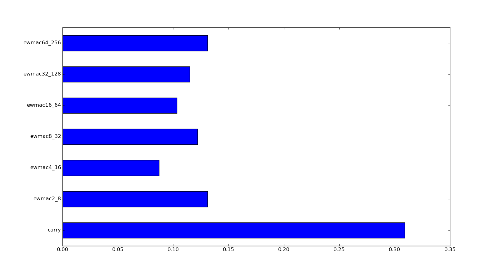
These two graphs are far more sensible. There is about 30% in carry in both; with pretty much equal weighting for the cheaper Eurostoxx market, and a tilt towards the cheaper variations for pricey V2X.
For the rest of this post I'll be using this combination.
Ignore gross returns, just use costs
forecast_cost_estimates:
use_pooled_costs: False
apply_cost_weight: False
ceiling_cost_SR: 999.0
cost_multiplier: 1.0
pool_gross_returns: True
equalise_gross: True
use_pooled_costs: False
use_pooled_turnover: True ## even when not pooling costs I recommend doing this
forecast_weight_estimate:apply_cost_weight: False
ceiling_cost_SR: 999.0
cost_multiplier: 1.0
pool_gross_returns: True
equalise_gross: True
 |
| Eurostoxx (cheap) |
 |
| V2X (expensive) |
Subtract costs from gross returns after multiply costs by a factor>1
forecast_cost_estimates:
use_pooled_costs: False
use_pooled_costs: False
use_pooled_turnover: True ## even when pooling I recommend doing this
forecast_weight_estimate:
apply_cost_weight: False
ceiling_cost_SR: 999.0
cost_multiplier: 3.0
pool_gross_returns: True
equalise_gross: False
apply_cost_weight: False
ceiling_cost_SR: 999.0
cost_multiplier: 3.0
pool_gross_returns: True
equalise_gross: False
 |
| Eurostoxx (Expensive) |
 |
| V2X (Cheap) |
Calculate weights using gross returns, and adjust subsequently for cost levels
forecast_cost_estimates:
use_pooled_costs: False
use_pooled_turnover: True ## even when pooling I recommend doing this
forecast_weight_estimate:apply_cost_weight: True
ceiling_cost_SR: 999.0
cost_multiplier: 0.0
pool_gross_returns: True
equalise_gross: False
 |
| EUROSTOXX (Cheap) |
 |
| V2X (Expensive) |
Apply a maximum cost threshold
forecast_cost_estimates:
use_pooled_costs: False
use_pooled_turnover: True ## even when pooling I recommend doing this
forecast_weight_estimate:apply_cost_weight: False
ceiling_cost_SR: 0.13
cost_multiplier: 1.0
pool_instruments: True
equalise_gross: False
 |
| EUROSTOXX (Cheap) |
 |
| V2X (Expensive) |
Really giving any allocation to ewmac2_8 has been kind of crazy because it is a rather expensive beast to trade. The V2X weighting is even more extreme removing all but the 3 slowest EWMAC variations. It's for this reason that chapter 15 of my book uses only these three rules plus carry.
My favourite setup
use_pooled_costs: False
use_pooled_turnover: True ## even when pooling I recommend doing this
forecast_weight_estimate:
apply_cost_weight: True
ceiling_cost_SR: 0.13
ceiling_cost_SR: 0.13
cost_multiplier: 0.0
pool_gross_returns: True
equalise_gross: False
As you'll know from reading my book I like the idea of culling expensive trading rules. This leaves the optimiser with less to do. I really like the idea of applying cost weighting (versus say multiplying costs my some arbitrary figure); which means optimising on gross returns. Equalising the returns before costs seems a bit extreme to me; I'd still like the idea of really poor trading rules being downweighted, even if they are the cheap ones. Pooling gross returns but using instrument specific costs strikes me as the most logical route to take.
 |
| Eurostoxx (cheap) |
 |
| V2X (expensive) |
A note about other optimisation methods
The other three methods in the package are shrinkage and one shot optimisation (just a standard mean variance). I don't recommend using the latter for reasons which I've mentioned many, many times before. However if you're using shrinkage be careful; the shrinkage of net return Sharpe Ratios will cancel out the effect of costs. So again I'd suggest using a cost ceiling, setting the cost multiplier to zero, then applying a cost weighting adjustment; the same setup as for bootstrapping.
forecast_cost_estimates:
use_pooled_costs: False
use_pooled_turnover: True ## even when pooling I recommend doing this
forecast_weight_estimate:
method: shrinkage
equalise_SR: False
ann_target_SR: 0.5
equalise_vols: True
shrinkage_SR: 0.90
shrinkage_corr: 0.50
apply_cost_weight: True
ceiling_cost_SR: 0.13
cost_multiplier: 0.0
pool_instruments: True
pool_costs: False
equalise_gross: False
forecast_cost_estimates:
use_pooled_costs: False
use_pooled_turnover: True ## even when pooling I recommend doing this
forecast_weight_estimate:
method: shrinkage
equalise_SR: Falseann_target_SR: 0.5
equalise_vols: True
shrinkage_SR: 0.90
shrinkage_corr: 0.50
apply_cost_weight: True
ceiling_cost_SR: 0.13
cost_multiplier: 0.0
pool_instruments: True
pool_costs: False
equalise_gross: False
ceiling_cost_SR: 0.13
cost_multiplier: 0.0
pool_instruments: True
pool_costs: False
equalise_gross: False
The Eurostoxx weights are very similar to those with bootstrapping. For V2X shrinkage ends up putting about 60% in carry with the rest split between the 3 slowest ewmac variations. This is more a property of the shrinkage method, rather than the costs. Perhaps the shrinkage isn't compensating enough for the uncertainty in the correlation matrix, which the bootstrapping does.
If you don't want to pool gross returns you might want to consider a higher shrinkage factor as there is less data (one of the reasons I don't like shrinkage is the fact the optimum shrinkage varies depending on the use case).
Instrument weights
In my book I actually suggested that ignoring costs for instrument trading subsystems is a perfectly valid thing to do. In fact I'd be pretty happy to equalise Sharpe ratios in the final optimisation and just let correlations do the talking.
Note that with instrument weights we also don't have the benefit of pooling. Also by using a ceiling on costs for trading rule variations it's unlikely that any instrument subsystem will end up breaking that ceiling.
Just for fun I ran an instrument weight optimisation with the same cost parameters as I suggested for forecasts. There is a smaller allocation to V2X and Eurostoxx; but that's probably because they are fairly highly correlated. One is the cheapest and the other the most expensive market, so the different weights are not driven by costs!
Key points from this post:
Happy optimising.
Note that with instrument weights we also don't have the benefit of pooling. Also by using a ceiling on costs for trading rule variations it's unlikely that any instrument subsystem will end up breaking that ceiling.
 |
| Instrument weights |
Summary
Key points from this post:
- Pooling gross returns data across instruments - good thing
- Using instrument specific costs - important
- Filtering out trading rules that are too expensive - very very important
- Using a post optimisation cost weighting - nice, but not a dealbreaker
- Using costs when estimating instrument weights - less important
Happy optimising.
This one requires some thought.
ReplyDeleteIf we were to just run the optimisation with our own config with NO mention of how costs are treated (e.g., no reference to 'apply_cost_weight', 'pool_costs', 'ceiling_cost', etc), what are the defaults that pysystemtrade reverts to?
The file systems.provided.defaults.yaml tells you this. eg
Deleteforecast_weight_estimate:
func: syscore.optimisation.GenericOptimiser
pool_instruments: True
pool_costs: False
equalise_gross: False
cost_multiplier: 0.0
apply_cost_weight: True
ceiling_cost_SR: 0.13
It's probably not a picture of Bayes but of an English churchman who lived about 100 years after Bayes. Rev. Bayes would have worn a wig in his portrait.
ReplyDeleteGlad I didn't say I was 100% sure. I'm bowled over by the erudite knowledge of the readers of this blog...
DeleteI am wondering for the optimisation.py in pyalgotrade. There are some adjustment factors (adj_factors) for the Sharpe Ratio difference. How are these calculated?
ReplyDeleteThey are from chapter 4 of my book.
DeleteHi Rob...just finished reading your book - my wife couldn't believe I was reading "a text book" after dinner as she rudely called your opus rather than watch Netflix!! Great stuff - finished it in two days and will go for a slower read through soon.
ReplyDeleteOne first thought that has bubbled up already, in terms of costs: would I be correct in thinking that selecting from high liquidity/tight spread ETFs with a US$2 round trip cost at IB (things like: SPY,GDX,EEM,XLF,EWJ,XIV,IWM,EFA,QQQ,FXI,USO,VWO,GDXJ,HYG,SLV,XLV,TLT) with the advantages of highly granular instrument blocks be acceptable in terms of meeting the trade cost requirements for something like the EWMAC 8,32 (and slower)?
I realise that for accounts above US$100K futures are always the way to go (refer https://www.peterlbrandt.com/trading-futures-forex-related-etfs-foolish-way-manage-trading-capital/ ) but for smaller accounts is my thinking on the right track?
Cheers, Donald
You are probably on the right track. Of those ETF I have only looked at SPY using the cost model in chapter 12 but it was certainly cheap enough to trade like a future.
DeleteMy second thought bubbling up, is would I be way off the "get to 10" concept if I did something like this?: use the read-outs from a Percent Price Oscillator, multiply each by 2 (this is for four EWMAVs), and cap at total of 20 (refer here for a qqq example http://schrts.co/Pgqbfg ) and here for more on the PPO ( http://bit.ly/2aFOCrx )
DeleteSo, to illustrate the "nitty-gritty", for QQQ at the moment, the PPOs read 1.758, 2.657, 2.904, 2.526 which sum to 9.845. Multiply this by 2, brings up to a current QQQ signal strength of 19.69
Regards, Donald
I am not familiar with the PPO. It doesnt seem to have a unitless scale. It will change scale in different vol enviroments. So I wouldn't use it.
DeleteHi Rob
DeleteAgreed.... ;-) I'm just on my second read through, and came across page 112 and page 160. These two make it very clear and easy to understand. The PPO fails in terms of not being proportional to expected risk adjusted returns...that's the whole enchilada right there, as the Americans might say!
By the way, thanks for putting together the excellent MS Excel files on the resource page....you've gone beyond the extra mile.
Cheers, Donald
...actually...on second thoughts, maybe not even bother with the multiplier of two. Just sum up the PPOs (and maybe ditch the fastest EWMAC as it's a bit quick for most things?).
ReplyDeleteHi Rob,
ReplyDeleteHow often do you rebalance cross-sectional strategies?
I don't have any
DeleteHi Rob,
ReplyDeleteIn your code there is a function named 'apply_cost_weighting'. If I debug the code with and using your data I receive following weight adjustment factors for the different rule variations :
- carry : 0.959611 (rule with lowest SR cost)
- ewmac16_64 : 0.990172
- ewmac32_128 : 0.976361
- ewmac4_16 : 1,141907 (rule with highest SR cost)
- ewmac64_256 : 0.969992
- ewmac8_32 : 1.036545
This result is the opposite from what I should expecting. I should expect that the cheapest rule gets the highest weight adj factor and the most expensive gets the lowest factor.
Is it possible that this rule :
relative_SR_costs = [cost - avg_cost for cost in ann_SR_costs]
should be
relative_SR_costs = [-1*cost - avg_cost for cost in ann_SR_costs] ?
Kris
no it should be working on returns not costs. bug fixed in latest release.
DeleteWith this new release the result looks fine, thnx
DeleteRob,
ReplyDeleteI've a question on bootstrapping in combination with pooling gross returns.
In pysystemtrade I see that you use bootstrapping based on random individual daily returns (also described in your book p 289). But as you mention on p 290, it's could be better to use 'block bootstrapping'.
For the pooling of the returns you stack up the returns by give them an extra second in the date-time field. After that you select random returns. But this isn't possible if we want to use block bootstrapping. I was thinking to work like this :
- get P&L from instrument 1
- get P&L from instrument 2
- get P&L from instrument 3
- stitch P&L of all this instruments :
--> P&L instrument 1 - P&L instrument 2 - P&L instrument 3
- create a virtual account curve from the stitched P&L's
- do block bootstrapping
Is this reasonable to do or do I overlook something ?
Kris
Yes, this is exactly right. You glue together the p&l so for example with 10 instruments of 10 years each you'd have a single 100 year long account curve. But this will make life complicated and may also run into problems with linux date storage. Instead keep the instruments in seperate buckets, say with 1 year blocks and 10 instruments each with 10 years of data you'd have 100 blocks (so populate a list of the blocks, rather than stitching). Then when you bootstrap pick N blocks at random with replacement from those 100 blocks; and stitch those together to create a set of data on which you run your single optimisation. Hope that makes sense.
DeleteYes this make sense and it's an interesting idea. I will try this out.
DeleteRob,
ReplyDeleteJust trying to get my head around the difference between
i) Calculate weights using gross returns, and adjust subsequently for cost levels
apply_cost_weight: True
cost_multiplier: 0
ii) using half-pooling
apply_cost_weight: False
cost_multiplier: 1.0
I only vaguely understand the difference and would appreciate more clarity!
Many thanks
Chris
i: optimisation is done without costs (pure pre-cost returns), and then the weights that come out are adjusted with more expensive assets seeing their weights reduced.
Deleteii: optimisation is done with post cost returns, but then weights aren't adjusted afterwards
Thanks
ReplyDeleteRob, I bought your book and in the process of replicating the logics to confirm my understanding. I have some questions regarding to cost estimation. I can grasp the standardised cost, i.e., SR for a round trip, yet I find it is confusing on the estimation of the turnover (for forecast level, instrument level and subsystem level)
ReplyDeleteIn your book, you used position level as example, and provided a formula as: average position change / 2 * average holding per year. Firstly, I do not understand why normalisation is required for this. If a round trip for a block value for an instrument costs 0.01 SR unit, and the number of block values changes says 10 round trip, doesn't this imply 0.01 * 10 = 0.10 SR unit, which should be subtracted from the expected return in various optimisation stage?
Furthermore, if I look into what is implemented in your python library, it seems that 2 * factor is missing (at least on the forecast level). Could you clarify this?
Thirdly, it is not clear how to include turnover estimation at forecast level as opposed to position level? Forecast generated is only proportional, not equal to estimated SR for a rule variation, wouldn't the cost estimation in the way you described in the book require to be scaled by an unknown factor?
As a separate note, on the carry strategy, for various future strategies, the front and back (2nd front) future are sufficient to use as proxy of carry, yet this is not true for commodity where seasonality could play a big role, I wonder how do you pick the right pair of future systematically? Moreover, is there a point to look at the how term structure?
"Firstly, I do not understand why normalisation is required "
DeleteIt's better to normalise and use SR of costs rather than actual $ figures or even percentages; because then you can easily compare costs across instruments and across time. In the absence of accurate figures for historic values of the bid-ask spread using vol normalised costs gives you a better approximation than assuming that current bid-ask spreads were realisable several decades ago.
"Furthermore, if I look into what is implemented in your python library, it seems that 2 * factor is missing" I'll look into this, issue is https://github.com/robcarver17/pysystemtrade/issues/61
Thirdly, it is not clear how to include turnover estimation at forecast level as opposed to position level?
Again, this is another reason to normalise cost. If you do this then you can just use the forecast turnover to calculate expected costs (though there may be further costs from changes in volatility affecting position size) multiplied by the SR of costs; and you don't need to worry about scaling factors.
4) yet this is not true for commodity where seasonality could play a big role,
See http://qoppac.blogspot.co.uk/2015/05/systems-building-futures-rolling.html
Thank you for your reply. The future rolling post is helpful. I had always been thinking the future liquidity is sole a monotonic (decreasing) function of the distance of maturity date.
DeleteAgain, this is another reason to normalise cost. If you do this then you can just use the forecast turnover to calculate expected costs (though there may be further costs from changes in volatility affecting position size) multiplied by the SR of costs; and you don't need to worry about scaling factors.
- Why won't I need to know deal with the scaling factor to calculate forecast turnover, but required to deal with a scaling factor (average annual position holding) is required for position turnover?
Thanks in advance
"- Why won't I need to know deal with the scaling factor to calculate forecast turnover, but required to deal with a scaling factor (average annual position holding) is required for position turnover?"
DeleteBecause forecasts are automatically scaled (average absolute value of 10), whereas the average absolute position value could be anything.
Hi Rob
ReplyDeleteIn your code you calculate raw forecast weights and afterwards you use an adjustment factor based on cost to change the weights. Also descriped in this article under 'Calculate weights using gross returns, and adjust subsequently for cost levels'
I've did some tests on this but my conclusion is that the adjustment factor is always low. This is normal because we eliminate rule variation with SR cost>0.13. This results in a very small adjustment on the raw weights.
If I recalculate the raw weights I see they vary for each calculation (which is normal I think) but I should expect that the adjustment factor should have a greater impact on the weights than recalculations.
Did you have experimented with bigger adjustment factors, so costs has a bigger impact on the raw weights ?
Kris
That's correct, and indeed it's something I note in my book - if you eliminate the high cost rules it's not worth bothering with adjustment.
DeleteThe adjustment factors are theoretically "correct" in the sense that they properly account for the appropriate adjustment given a situation in which you know the sharpe ratio difference with something close to certainty. Experimenting with them would be akin to fitting yet another parameter, in sample, and so a horrendously bad thing.
Rob,
ReplyDeleteI have noted that when using pysystem on collections of shares such as ETF's and particularly unit trusts that the cost ceiling of SR-turnover of 0.13 is very restrictive on account of the lower volatility of these grouped instruments.
If one wanted to use these vehicles, would it be better to increase the cost ceiling to say 1.5 or set apply_cost_weight: False and cost_multiplier: 1?
Thanks
Chris
No, it would be better to slow down your trading considerably :-)
DeleteHi Rob,
ReplyDeleteI saw that on page 196 of Systematic Trading, third para, you indicate that we can approximate turnover of combined forecasts by taking the weighted average turnover of the individual forecasts. I assume this is in fact intended as a means to get a quick approximation as I would think the 'turnover of the weighted average forecasts' to be lower than the 'weighted average of the individual turnovers' (due to imperfect correlation)? As a crosscheck, tentatively, I think I managed to verify this via a quick comparison using random returns data.
Yes you're right about this being an approximation.
DeleteThank you Rob. With regard to estimating expected turnover for a each rule variation, rather than using real data, I wonder if it is best to fix these simply with the help of simulated gaussian returns? Otherwise, if we are removing rules based on speed thresholds, and if estimated speeds vary as we change our window of observations, it is possible to end up with changing rule sets for an instrument over time and in different backtests. Could be done but it seems overkill and also I personally can't see why expected turnover should vary over time for a given rule. I am probably preaching to the converted in CH3, I get the impression this is exactly what you recommend doing?
DeleteAs you can see I am still thoroughly enjoying (re) reading your excellent book.
Using random data to estimate turnover is an excellent idea, and one I have talked about (i.e https://www.youtube.com/watch?v=s2NSlxHq6Bc ) and blogged about (https://qoppac.blogspot.co.uk/2015/11/using-random-data.html).
DeleteFantastic presentation, thanks. So I am now trying to recreate trending markets at different frequencies. Question I have is how to superimpose noise on the sawtooth. The sawtooth is the cumsum of all drift terms, so noise should also be the cumsum of noise?
Deletehttps://github.com/robcarver17/systematictradingexamples/blob/master/commonrandom.py
DeleteThanks Rob, I have looked at your spreadsheet here https://tinyurl.com/ycs8lmp3 and the github code and as far as I can tell they seem to be generating different price processes. The code produce a price path with gaussian 'error' overlayed, whereas the spreadsheet produces a price path along the lines what I think I stated above which is the cumulative(drift + error). I don't know if the code needs correcting or the spreadsheet.
DeleteI think the spreadsheet is correct - the graphs look more realistic.
DeleteThis comment has been removed by the author.
DeleteWell, this is interesting, if I have done things correctly. Using simulated data, if I use a volscale of ~ 0.16 (to amplitude) and take out the fastest and slowest rules plus focus only on trend frequencies of 1-6 pa, turnover doesn't vary that much (still varies more than I would expect). However when I lower the volscale to 0.02 and look at wider ranges, turnover varies quite a bit. Taking the ewmac2,8 as an example and looking at a trend frequency from once every three years to once a month, the turnover falls from 57 to 18. Its also slightly counterintuitive to me that turnover would fall if trend frequency goes up. Could this be correct? I could have done something fatally wrong, but if not, would it be correct to think that simulated turnover has some limitations (given that I have no idea what the correct 'harmonic frequency', as you put it, will be). Happy to send across a small table of results by email or through whatever channel which might allow formatted tables to be read easily.
ReplyDeleteIt does sound weird. I have done a similar exercise but I can't remember what range of volscale I used. I didn't do it very scientifically but if I toned the vol scale down too much then I stopped seeing 'realistic' looking price series (and also the Sharpe Ratio of the ewmac pairs became unrealistically high). I haven't really got time to dig into this, but my approach was basically to generate some results with simulated data and then check they were roughly in the right ball park with real price data.
DeleteThis comment has been removed by the author.
DeleteThanks and understood. I agree it can be time consuming. My initial starting point was that volscales could vary enormously depending on the market (0.02 is about right for a market whose trend amplitude shows doubling and halving which some commodity markets can display), whereas 0.2 is right for markets with usual shallower trends. This in turn seems to result in wide turnover ranges. I will see if I can come with an alternative formulation of trend patterns and see if that makes the outcomes more stable.
DeleteP.S. To quote Gene Hackman in the movie 'Heist': 'I am burnt..', but somehow the movie survives with the fiction that he is not, and I shall try to continue with that fiction, if that's OK)
Hi Rob,
ReplyDeleteI am trying to calculate the SR drag and account curve degradation from costs in my backtests.
From reading Chapter Twelve and this blogppost, I understand that the expected annual SR drag can be estimated by using SR unit cost and normalised annual turnover. After some effort in trying to understand maths behing the normalisation of turnover, it appears to me that the turnover normalisation factor (volscalar) relies on the assumption that the system is consistently meeting its vol targets. If it is not, would I be correct in adjusting normalisation factor by the realised vol to get a slightly more accurate picture of SR drag in my system over time, particularly as realised vol can vary quite a bit over time? Of course, I recognise the historic SR estimate is in itself subject to considerable error, so it is a moot point whether this correction would enormous value in itself.
You're right; I don't think this would add any value at all :-)
DeleteHarsh. But fair :)
DeleteHi Rob, I intend to use some of the code you've shared here. In order to use this, I guess I have to add my broker's per trade commission in the rightmost column ("Per Trade") of the instrumentconfig.csv file found here C:\pysystemtrade-master\data\futures\csvconfig. Is that correct? Thanks.
ReplyDeleteYes if you're commission is PER TRADE, and not PER BLOCK. So for example if you pay a flat fee of $10 per trade regardless of size. But if you get charged say $1 per 100 shares, or $1 per futures contract, then it goes in the 'per block' place. Having said all that I'm not sure if pysystemtrade deals correctly with per trade costs - it's been a while since I wrote that part of the code.
DeleteHi Rob, please allow me ask 2 questions, regarding the trading rule weighting:
ReplyDelete1) Do you still use fast trading rules, i.e., ewmac2_8, ewmac4_16, breakout10, breakout 20? I had the impression that you don't, accoding to what you said in TopTraderUnplugged Podcast, and the EliteTrader posts. I am considering removing them for all instruments, although my caclulation says we can use them for the cheapest instruments, as I feel I am trading more often than I should. Just feeling though.
2) Do you think reducing weight for carry rule from 50% (my current weight) to 33% (new weight I just implemented this moring) a bad idea? I observed that you said your carry weight is aroud 20%-30% (same sources as #1). The reason for the change was that I noticed that the carry forecasts tend to have extreme scores compared to the ewmac and breakout. I got -20 scores for 5yr bonds, vol, and meat, consistently for almost all the carry variations (variation by smoothing period). And +20 scores for 10yr bonds, corn and soybean. I suspected I did something wrong with my carry calculation, but it looks OK. Those instruments seem to have big negative or positive carry. However in my very limited trading experience (only 2 months!), I don't feel I have been rewarded by betting on the carry.
I wish I could run backtesting myself. Sadly my skill is not high enough, and I still cannot make pysystemtrade work. I am sure I will soon be able to, as I believe I am learning fairly quickly in the last couple of months since I started the futures trading trial (with real money!). Thanks!
I will allow :-)
Delete1) I do use them although the weights are pretty low, and even then only in cheap instruments like S&P 500 the total weight for those 4 rules is just 3% so dropping them completely wouldn't make much difference.
If you're using buffering to reduce trading, then removing very fast rules without much weight probably won't change your trading costs very much.
2) You're right that carry is often more extreme than momentum (which has a natural distribution closer to normal, especially slower momentum) although I'd argue that judged over long time periods it's better behaved. Scanning through my current forecasts I can see some extremes for carry, but also for quite a few momentum signals.
Notice also that if carry is symmetric, then even if it was more extreme it would still have the same average contribution to risk that it's forecast weight suggested (this would be the case even if it was binary).
Is reducing the weight to carry a bad idea? Not neccessarily. It depends on if you are doing it for the right reasons. If you're doing it because you think the signal is contributing more to risk than it's forecast weight suggests, then reduce it (although again I'd caution that probably isn't the case).
If you're doing it because you only have a single carry rule, and thus it's effectively over represented on a risk contribution basis compared to multiple trend following rules, then it's fine (but the easy fix to this is to do what I do, and trade several different versions of carry with different smooths of the raw carry signal).
However when you say "in my very limited trading experience (only 2 months!), I don't feel I have been rewarded by betting on the carry." I get very worried because you're basically throwing away a fit based on decades of data based on a hunch and a very short period of time....
"and I still cannot make pysystemtrade work" Ah don't worry there are days when I can't make it work eithier (the development branch, not the stable version!) I'm doing my best to get to version 1.0 which will hopefully be more robust and accessible.
Hi Rob! Thank you for the answers!
DeleteI cannot help asking follow up questions...
Buffering: I see my "10% buffering" works effectively for instruments of rather big positions (e.g., >5), but it does not for those of small positions (e.g., <5), because of the fraction problem. Is my implementation wrong?
Weight for carry rules: What is your basis behind for allocating around 30% for carry rules? You said your allocation was like 60% trend follow, 30% carry, and 10% something else.
You are right, thowing away the fit over decades of data does not sound a good thing. Also I am convinced with the symmetry aspect answer. I am finding it rather difficult to behave scientific and logical, particularly when real money is involved...
Looking forward to the version 1.0 of the pysystemtrade! (although it is very likely that the reason for the difficulty I am facing is simply due to my lack of skills)
>Buffering: I see my "10% buffering" works effectively for instruments of rather big positions (e.g., >5), but it does not for those of small positions (e.g., <5), because of the fraction problem. Is my implementation wrong?
DeleteNot it's logical that buffering will have less effect when positions are smaller.
>Weight for carry rules: What is your basis behind for allocating around 30% for carry rules? You said your allocation was like 60% trend follow, 30% carry, and 10% something else.
It's pretty much what my handcrafted optimisation method comes up with.
Thank you! I got clearer picture now. Actually the handcrafting post is something I will deep read and try myself in this weekend. I am expecting to find more reasonable instrument allocation (yes instrument allocation) than my current portfolio. Thanks!
DeleteOne last comment before I forget. I thought it would look nicer if the scalars for the breakout were "40". With this, I believe the breakout scores have the same range of +/- 20, as other rules do.
DeleteWhen I first looked at the breakout forecast scores my very poor code generates for the first time, I thought I made something wrong. I saw many 14.3 or 16.8 or similar, but no higher. They were just half the number of the scalar you recommend in your book! I triple checked your book, and comfirmed that it is OK, since I finally find you rightly say that the raw breakout forecast scores before multipling the scalar has fixed range of +/-0.5. I thought until recently that the scalars were defined that way such that the equal weight across the time variations make sence. Now that you give different weights to different time variations, you do not need to worry about it any longer I suppose.
Hi Rob! Regarding my comment above for forecast scalars for breakout, I just found your blog post where you did use "40" for breakout scalar (https://qoppac.blogspot.com/2016/05/a-simple-breakout-trading-rule.html). Somehow I overlooked the post until now, and had only referenced Leveraged Trading in my comment above...sorry about that. I will revise my codes accordingly. Thank you!
DeleteHi Rob,
ReplyDeleteStill new to pysystemtrade but the example code "optimisation with costs" you mentioned https://github.com/robcarver17/pysystemtrade/blob/master/examples/optimisation/optimisationwithcosts.py
seemed to have been moved to
https://github.com/robcarver17/pysystemtrade_examples/blob/master/optimisation/optimisationwithcosts.py
which has dependencies on pysystemtrade. However there seems no "bootstrap" method implemented anymore in pysystemtrade, therefore the code doesn't run and throws "Optimiser bootstrap not recognised".
Thanks
Hi Rob,
ReplyDeletei've seen that the defaults in defaults.yaml have changed versus what you mentioned in a previous post and also form what you mentioned was your favuorite setup in this article:
defaults now
cost_multiplier: 2.0
apply_cost_weight: False
ceiling_cost_SR: 9999
your favorite setup:
cost_multiplier: 0.0
apply_cost_weight: True
ceiling_cost_SR: 0.13
has something changed that made you think that today's defaults are "better"?
thanks
Not really. There isn't much in it to be honest I just play with them occasionally.
Delete