As you might expect I spend quite a lot of my time using real financial data - asset prices and returns; and returns from live and simulated trading. It may surprise you to know that I also spend time examining randomly created financial data.
This post explains why. I also explain how to generate random data for various purposes using both python and excel. I'll then give you an example of utilising random data; to draw conclusions about drawdown distributions and other return statistics.
This is the first in a series of three posts. I intend to follow up with three more posts illustrating how to use random data - the second will be on 'trading the equity curve' (basically adjusting your system risk depending on your current performance), and the third illustrating why you should use robust out of sample portfolio allocation techniques (again covered in chapter 4 of my book).
Why random data is a good thing
As systematic traders we spend a fair amount of our time looking backwards. We look at backtests - simulations of what would have happened if we ran our trading system in the past. We then draw conclusions, such as 'It would have been better to drop this trading rule variation as it seems to be highly correlated with this other one', or 'This trading rule variation holds it's positions for only a week', or 'The maximum drawdown I should expect is around 20%' or 'If I had stopped trading once I'd lost 5%, and started again once I was flat, then I'd make more money'.
However it is important to bear in mind that any backtest is to an extent, random. I like to think of any backtest that I have ran as a random draw from a massive universe of unseen back tests. Or perhaps a better way of thinking about this is that any financial price data we have is a random draw from a massive universe of unseen financial data, which we then run a backtest on.
This is an important concept because any conclusions you might draw from a given backtest are also going to randomly depend on exactly how that backtest turned out. For example one of my pet hates is overfitting. Overfitting is when you tune your strategy to one particular backtest. But when you actually start trading you're going to get another random set of prices, which is unlikely to look like the random draw you had with your original backtest.
As this guy would probably say, we are easily fooled by randomness:
 |
| Despite his best efforts in the interview Nassim didn't get the Apple CEO job when Steve retired. Source: poptech.org |
In fact really every time you look at an equity curve you ought to draw error bars around each value to remind you of this underlying uncertainty! I'll actually do this later in this post.
There are four different ways to deal with this problem (apart from ignoring it of course):
- Forget about using your real data, if you haven't got enough of it to draw any meaningful conclusions
- Use as many different samples of real data as possible - fit across multiple instruments and use long histories of price data not just a few years.
- Resample your real data to create more data. For example suppose you want to know how likely a given drawdown is. You could resample the returns from a strategies account curve, see what the maximum drawdown was, and then look at the distributions of those maximum drawdowns to get a better idea. Resampling is quite fun and useful, but I won't be talking about it today.
- Generate large amounts of random data with the desired characteristics you want, and then analyse that.
This post is about the fourth method. I am a big fan of using randomly generated data as much as possible when designing trading systems. Using random data, especially in the early stages of creating a system, is an excellent way to steer clear of real financial data for as long as possible, and avoid being snared in the trap of overfitting.
The three types of random data
There are three types of random data that I use:
- Random price data, on which I then run a backtest. This is good for examining the performance of individual trading rules under certain market conditions. We need to specify: the process that is producing the price data which will be some condition we like (vague I know, but I will provide examples later) plus Gaussian noise.
- Random asset returns. The assets in question could be trading rule variations for one instrument, or the returns from trading multiple instruments. This is good for experimenting with and calibrating your portfolio optimisation techniques. We need to specify: The Sharpe ratio,standard deviation and correlation of each asset with the others.
- Random backtest returns for an entire strategy. The strategy that is producing these returns is completely arbitrary. We need to specify: The Sharpe ratio, standard deviation and skew of strategy returns (higher moments are also possible)
Notice that I am not going to cover in this post:
- Price processes with non Gaussian noise
- Generating prices for multiple instruments. So this rules out testing relative value rules, or those which use data from different places such as the carry rule. It is possible to do this of course, but you need to specify the process by which the prices are linked together.
- Skewed asset returns (or indeed anything except for a normal, symmettric Gaussian distribution). Again in principle it's possible to do this, but rather complicated.
- Backtest returns which have ugly kurtosis, jumps, or anything else.
In an abstract sense then we need to be able to generate:
- Price returns from some process plus gaussian noise (mean zero returns) with some standard deviation
- Multiple gaussian asset returns with some mean, standard deviation and correlation
- Backtest returns with some mean, standard deviation and skew
Generating random data
Random price data
To make random price series we need two elements: an underlying process and random noise. The underlying process is something that has the characteristics we are interested in testing our trading rules against. On top of that we add random gaussian noise to make the price series more realistic.
The 'scale' of the process is unimportant (although you can scale it against a familiar asset price if you like), but the ratio of that scale to the volatility of the noise is vital.
Underlying processes can take many forms. The simplest version would be a flat line (in which case the final price process will be a random walk). The next simplest version would be a single, secular, trend. Clearly the final price series will be a random walk with drift. The process could also for example be a sharp drop.
Rather than use those trivial cases the spreadsheet and python code I've created illustrate processes with trends occuring on a regular basis.
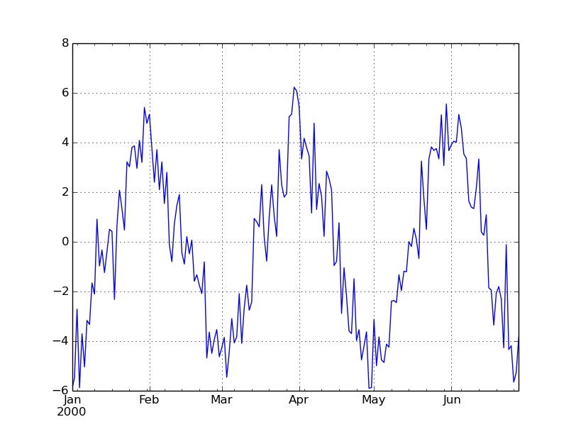
Using the python code here is the underlying process for one month trends over a 6 month period (Volscale=0.0 will add no noise, and so show us the underlying process):
ans=arbitrary_timeseries(generate_trendy_price(Nlength=180, Tlength=30, Xamplitude=10.0, Volscale=0.0)).plot()

Here is one random series with noise of 10% of the amplitude added on:
ans=arbitrary_timeseries(generate_trendy_price(Nlength=180, Tlength=30, Xamplitude=10.0, Volscale=0.10)).plot()
And here again another random price series with five times the noise:
ans=arbitrary_timeseries(generate_trendy_price(Nlength=180, Tlength=30, Xamplitude=10.0, Volscale=0.50)).plot()

Random correlated asset returns
Spreadsheet: There is a great resource here; others are available on the internet
My python code is here
It's for three assets but you should be able to adapt it easily enough.
Here is an example of the python code running. Notice the code generates returns, these are cumulated up to make an equity curve.
SRlist=[.5, 1.0, 0.0]
clist=[.9,.5,-0.5]
threeassetportfolio(plength=5000, SRlist=SRlist, clist=clist).cumsum().plot()

Random backtest returns (equity curve) with skew
Spreadsheet: There are a number of resources on the internet showing how skewed returns can be generated in excel including this one.
My python code
From my python code here is an equity curve with an expected Sharpe Ratio of +0.5 and no skew (gaussian returns):
cum_perc(arbitrary_timeseries(skew_returns_annualised(annualSR=0.5, want_skew=0.0, size=2500))).plot()

Now the same sharpe but with skew of +1 (typical of a relatively fast trend following system):
cum_perc(arbitrary_timeseries(skew_returns_annualised(annualSR=0.5, want_skew=1.0, size=2500))).plot()

Here is a backtest with Sharpe 1.0 and skew -3 (typical of a short gamma strategy such as relative value fixed income trading or option selling):
cum_perc(arbitrary_timeseries(skew_returns_annualised(annualSR=1.0, want_skew=-3.0, size=2500))).plot()

We'll use this python code again in the example at the end of this post (and in the next post on trading the equity curve).
Safe use of random data
What can we use random data for?
Some things that I have used random data for in the past include:
- Looking at the correlation of trading rule returns
- Seeing how sensitive optimal parameters are over different backtests
- Understanding the likely holding period, and so trading costs, of different trading rules
- Understanding how a trading rule will react to a given market event (eg 1987 stock market crash being repeated) or market environment (rising interest rates)
- Checking that a trading rule behaves the way you expect - picks up on trends of a given length, handles corners cases and missing data, reduces positions at a given speed for a reversal of a given severity
- Understanding how long it takes to get meaningful statistical information about asset returns and correlations
- Understanding how to use different portfolio optimisation techniques; for example if using a Bayesian technique calibrating how much shrinkage to use (to be covered in the final post of this series)
- Understanding the likely properties of strategy account curves (as in the example below)
- Understanding the effects of modifying capital at risk in a drawdown (eg using Kelly scaling or 'trading the equity curve' as I'll talk about in the next post in this series)
What shouldn't we use random data for?
Random data cannot tell you how profitable a trading rule was in the past (or will be in the future... but then nothing can tell you that!). It can't tell you what portfolio weights to give to instruments or trading rule variations. For that you need real data, although you should be very careful - the usual rules about avoiding overfitting, and fitting on a pure out of sample basis apply.
Random data in a strategy design workflow
Bearing in mind the above I'd use a mixture of random and real data as follows when designing a trading strategy:
- Using random data design a bunch of trading rule variations to capture the effects I want to exploit, eg market trends that last a month or so
- Design and calibrate method for allocating asset weights with uncertainty, using random data (I'll cover this in the final post of this series)
- Use the allocation method and real data to set the forecast weights (allocations to trading rule variations) and instrument weights; on a pure out of sample basis (eg expanding window).
- Using random data decide on my capital scaling strategy - volatility target, use of Kelly scaling to reduce positions in a drawdown, trade the equity curve and so on (I'll give an example of this in the next post of this series).
Example: Properties of back tested equity curves
To finish this post let's look at a simple example. Suppose you want to know how likely it is that you'll see certain returns in a given live trading record; based on your backtest. You might be interested in:
- The average return, volatility and skew.
- The likely distribution of daily returns
- The likely distribution of drawdown severity
- We know roughly what sharpe ratio to expect (from a backtest or based on experience)
- We know roughly what skew to expect (ditto)
- We have a constant volatility target (this is arbitrary, let's make it 20%) which on average we achieve
- We reduce our capital at risk when we make losses according to Kelly scaling (i.e. a 10% fall in account value means a 10% reduction in risk; in practice this means we deal in percentage returns)
Let's go through the python code and see what it is doing (some lines are missed out for clarity). First we create 1,000 equity curves, with the default annualised volatility target of 20%. If your computer is slow, or you have no patience, feel free to reduce the number of random curves.
length_backtest_years=10
number_of_random_curves=1000
annualSR=0.5
want_skew=1.0
random_curves=[skew_returns_annualised(annualSR=annualSR, want_skew=want_skew, size=length_bdays)
for NotUsed in range(number_of_random_curves)]
We can then plot these:
plot_random_curves(random_curves)
show()

All have an expected Sharpe Ratio of 0.5, but over 10 years their total return ranges from losing 'all' their capital (not in practice if we're using Kelly scaling), to making 3 times our initial capital (again in practice we'd make more).
The dark line shows the average of these curves. So on average we should expect to make our initial capital back (20% vol target, multiplied by Sharpe Ratio of 0.5, over 10 years). Notice that the cloud of equity curves around the average gives us an indication of how uncertain our actual performance over 10 years will be, even if we know for sure what the expected Sharpe Ratio is. This picture alone should convince you of how any individual backtest is just a random draw.
* Of course in the real world we don't know what the true Sharpe Ratio is. We just get one of the lighted coloured lines when we run a backtest on real financial data. From that we have to try and infer what the real Sharpe Ratio might be (assuming that the 'real' Sharpe doesn't change over time ... ). This is a very important point - never forget it.
Note that to do our analysis we can't just look at the statistics of the black line. It has the right mean return, but it is way too smooth! Instead we need to take statistics from each of the lighter lines, and then look at their distribution.
Magic moments
Mean annualised return
function_to_apply=np.mean
results=pddf_rand_data.apply(function_to_apply, axis=0)
## Annualise (not always needed, depends on the statistic)
results=[x*DAYS_IN_YEAR for x in results]
hist(results, 100)

Volatility
function_to_apply=np.std
results=pddf_rand_data.apply(function_to_apply, axis=0)
## Annualise (not always needed, depends on the statistic)
results=[x*ROOT_DAYS_IN_YEAR for x in results]
hist(results, 100)

But all those things apply equally to the mean - and that is still extremely unstable even in the simplified random world we're using here.
Skew
import scipy.stats as st
function_to_apply=st.skew
results=pddf_rand_data.apply(function_to_apply, axis=0)
hist(results, 100)

Skew is also relatively stable (in this simplified random world). I plotted this to confirm that the random process I'm using is reproducing the correct skew (in expectation).
Return distribution
function_to_apply=np.percentile
function_args=(100.0/DAYS_IN_YEAR,)
results=pddf_rand_data.apply(function_to_apply, axis=0, args=function_args)
hist(results, 100)

Drawdowns
Average drawdown
results=[x.avg_drawdown() for x in acccurves_rand_data]
hist(results, 100)

Really bad drawdowns
results=[x.worst_drawdown() for x in acccurves_rand_data]
hist(results, 100)

Clearly I could continue and calculate all kinds of fancy statistics; however I'm hoping you get the idea and the code is hopefully clear enough.
What's next
As promised there will be two more posts in this series. In the next post I'll look at using random backtest returns to see if 'trading the equity curve' is a good idea. Finally I'll explore why you should use robust portfolio optimisation techniques rather than any alternative.
Thanks for calling my blogpost a "great resource"! Appreciate it!
ReplyDeleteYou're welcome Kurt.
DeleteHi Rob,
ReplyDeleteWhen I build new trading rule, Why I need simulate the signal + noise( Hard for more complex rules). Is it possible to generate blook bootstrap from time series (CL,EURUSD ...) to preserve the relations instead of simulating the signal?
Yes, but (a) you'll be using real data - which means potentially overfitting and using forward looking information (eg if your backtest is in 1980 but using a block from 1995), (b) blocks have to be long enough to capture the term structure of autocorrelation you want to model, (c) what do you do when blocks join up?
DeleteYou might as well do something simpler - take each year of your data in the past so far (at that point in the backtest), fit your rule to each year, and then take the average of the parameters fitted over various years.
Hi Rob,
ReplyDeleteThanks for the post. How would you use random data when the trading rule depends on another data source? For example, trade index future based on non farm payroll results. In this instance would you need to generate random data for index future prices and non farm payroll data and assume some correlation between them?
So what you're doing is 'assuming my rule works, let me check to see if my rule works'.... not sure what the point of that is??
Delete