Tuesday, 10 November 2015

Random data: Evaluating "Trading the equity curve"

Everyone hates drawdowns (those periods when you're losing money whilst trading). If only there was a way to reduce their severity and length....

Quite a few people seem to think that "trading the equity curve" is the answer. The basic idea is that when you are doing badly, you reduce your exposure (or remove it completely) whilst still tracking your 'virtual' p&l (what you  would have made without any interference). Once your virtual p&l has recovered you pile back into your system. The idea is that you'll make fewer losses whilst your system is turned off. It sounds too good to be true... so is it? The aim of this post is to try and answer that question.

This is something that I have looked at in the past, as have others, with mixed results. However all the analysis I've seen or done myself has involved looking at backtests of systems based on actual financial data. I believe that to properly evaluate this technique we need to use large amounts of random data, which won't be influenced by the fluke of how a few back tests come out. This will also allow us to find which conditions will help equity curve trading work, or not.

This is the second post in a series on using random data. The first post is here.
 

How do we trade the equity curve?


I'm going to assume you're reasonably familiar with the basic idea of equity curve trading. If not, then its probably worth perusing this excellent article from futures magazine.

An equity curve trading overlay will comprise of the following components:

  • A way of identifying that the system is 'doing badly', and quantifying by how much.
  • A rule for degearing the trading system given how badly it is doing
  • A second rule for regearing the system once the 'virtual' account curve is 'doing better'

I've seen two main ways for identifying that the system is doing badly. The first is to use a straightforward drawdown figure. So, for example, if your drawdown exceeds 10% then you might take action.

(Sometimes rather than the 'absolute' drawdown, the drawdown since the high in some recent period is considered)

The second variation is to use a moving average (or some other similar filter) of the account curve. If your account curve falls below the moving average, then you take action.

(There are other variations out there, in particular I noticed that the excellent  Jon Kinlay blog had a more complex variation)

As for degearing your system, broadly speaking you can eithier degear it all in one go, or gradually. Usually if we dip below the moving average of an equity curve then it is suggested that you cut your position entirely.

Whilst if you are using the current drawdown as your indicator, then you might degear gradually: drawdown; then by another 20% for a total of 40% when you hit a 20% drawdown and so on.

Note that this degearing will be in addition to the normal derisking you should always do when you lose money; if you lose 10% then you should derisk your system by 10% regardless of whether you are using an equity curve trading overlay.

Finally the 'regearing' rule is normally the reverse of the degearing rule and process. 


Prior research


The idea of trading the equity curve is something that seems to have bypassed academic researchers (unless they are calling it something else - please write in if you know about any good research) so rather than any formal literature review I had a quick look at the first page of google.

Positive


adaptrade
crazy ivan (whether he's a reliable source I don't know...)
Jon Kinlay (though not the normal system)


Negative (or at least no clear benefit)


Futures magazine (and also here)
Anthony Garnett
futures.io
r-bloggers


Why random data?


I personally find the above research interesting, but not definitive one way or another. My main issue is that it was all done on different financial instruments and different kinds of trading systems, which unsuprisingly gave different results. This might be because there is something 'special' about those instruments where equity curve trading worked, but it's more likely to be just dumb luck. Note: It is slightly more plausible that different kinds of trading rules will give different results; and we'll explore this below.

I personally think that we can't properly evaluate this kind of overlay without using random data. By generating returns for different arbitrary trading strategies we can then judge whether on average equity curve trading will be better.

Another advantage of using random data to evaluate an equity curve overlay system is that we avoid potentially overfitting. If we run one version of the overlay on our system, and it doesn't work, then it is very tempting to try a different variation until it does work. Of course we could 'fit' the overlay 'parameters' on an out of sample basis. But this quite a bit of work; and we don't really know if we'd have the right parameters for that strategy going forward or if they just happened to be the best for the backtest we ran.

Finally using random data means we can discover what the key characteristic of a trading system is that will allow trading the equity curve to work, or not.


Designing the test


Which overlay method?


There are probably an infinite variety of methods of doing an equity curve trading overlay (of which I touched on just a few above). However to avoid making this already lengthy post the size of an encylopedia I am going to limit myself to testing just one method. In any case I don't believe that the results for other methods will be substantially different.

I'm going to focus on the most popular, moving average, method:

 "When the equity curve falls below it's N day moving average, turn off the system. Keep calculating the 'virtual' curve, and it's moving average during this period. When the 'virtual' curve goes back above it's moving average then turn the system back on"

That just leaves us with the question of N.  Futures magazine uses 10, 25 and 40 days and to make life simple I'll do the same. However to me at least these seem incredibly short periods of time. For these faster N trading costs may well overwhelm any advantage we get (and I'll explore this later).

Also wouldn't it be nice to avoid the 3 year drawdown in trend following that happened between 2011 and 2013? Because we're using random data (which we can make as long as we like) we can use longer moving averages which wouldn't give us meaningful results if we tested just a few account curves which were 'only' 20 years long.

So I'll use N=10, 25, 40, 64, 128, 256, 512

(In business days; 2 weeks, 5 weeks, 8 weeks, 3 months, 6 months, 1 year, 2 years)

def isbelow(cum_x, mav_x, idx):
 

    ## returns 1 if cum_x>mav_x at idx, 0 otherwise
 

    if cum_x[idx]>=mav_x[idx]:
        return 1.0
    return 0.0
 

def apply_overlay(x, N_length):
    """
    apply an equity curve filter overlay
   
    x is a pd time series of returns
   
    N_length is the mav to apply
   
    Returns a new x with 'flat spots'
   
    """
    if N_length==NO_OVERLAY:
        return x

    cum_x=x.cumsum()
    mav_x=pd.rolling_mean(cum_x, N_length)
    filter_x=pd.TimeSeries([isbelow(cum_x, mav_x, idx) for idx in range(len(x))], x.index)
   
    ## can only apply with a lag (!)
    filtered_x=x*filter_x.shift(1)


    return filtered_x


Which criteria?


A nice way of thinking about equity curve trading is that it is a bit like buying insurance, or in financial terms a put option on your system's performance. If your system does 'badly' then the insurance policy prevents you from losing too much.

One of my favourite acronyms is TINSTAAFL. If we're buying insurance, or an option, then there ought to be a cost to it. Since we aren't paying any kind of explicit premium, the cost must come in the form of losing something in an implicit way. This could be a lower average return, or something else that is more subtle. This doesn't mean that equity curve trading is automatically a bad thing - it depends on whether you value the lower maximum drawdown* more than the implicit premium you are giving up.

* This assumes we're getting a lower maximum drawdown - as we'll see later this isn't always the case.

I can think of a number of ways of evaluating performance which try and balance risk and reward. Sadly the most common, Sharpe Ratio, isn't appropriate here. The volatility of the equity curve with the overlay on will be, to use a technical term, weird - especially for large N. Long periods without returns will be combined with periods when return standard deviation is normal. So the volatility of the curve with an overlay will always be lower; but it won't be a well defined statistic. Higher statistical moments will also suffer.

Instead I'm going to use the metric return / drawdown. To be precise I'm going to see what effect adding the overlay has on the following account curve statistics:

  • Average annual return
  • Average drawdown
  • Maximum drawdown
  • Average annual return / average drawdown
  • Average annual return / maximum drawdown
(Note that return / drawdown is a good measure of performance as it is 'scale invarient'; if you double your leverage then this measure will be unchanged)

My plan is to generate a random account curve, and then measure all the above. Then I'll pass it through the equity overlay, and remeasure the statistics.

Finally just to note that for most of this post I won't be considering costs. For small N, given we are closing our entire strategy down and then restarting it potentially every week, these could be enormous. Towards the end I will give you an idea of how sensitive the findings are to the costs of different trading instruments.


Which equity curve characteristics?


Broadly speaking the process for using random data is:

  • Identify the important characteristics of the real data you need to model
  • Calibrate against some real data
  • Create a process which produces random data with the neccessary characteristics
  • Produce the random data, and then do whatever it is you need to do

Notice that an obvious danger of this process is making random data that is 'too good'. In an extreme case with enough degrees of freedom you could end up producing 'random' data which looks exactly like the data you calibrated it against! There is a balance between having random data that is realistic enough for the tests you are running, and 'over calibrated'.


Identification


What characteristics of a trading system returns will affect how well an equity curve overlay will work? As in my previous post I'll be producing returns that have a particular volatility target - that won't affect the results.

They will also have a given expected Sharpe Ratio. With a negative Sharpe Ratio equity curve overlay should be fantastic - it will turn off the bad system. With a high positive Sharpe Ratio they will probably have no effect (at least for large enough N). It's in the middle that things will get more interesting. I'll test Sharpe Ratios from -2 to +2.

My intuition is that skew is important here. Negative skew strategies could see their short, sharp, losses reduced. Positive skew such as trend following strategies which tend to see slow 'bleeds' in capital might be improved by an overlay (and this seems to be a common opinion amongst those who like these kind of systems). I'll test skew from -2 (average for a short volatility or arbitrage system) to +1 (typical of a fast trend following system).

Finally I think that autocorrelation of returns could be key. If we tend to get losses one after the other then equity curve trading could help turn off your system before the losses get too bad.


Calibration


First then for the calibration stage we need some actual returns of real trading systems.

The systems I am interested in are the trading rules described in my book, and in this post: a set of trend following rule variations (exponentially weighted moving average crossover, or EWMAC for short) and a carry rule.

First skew. The stylised fact is that trend following, especially fast trend following, is positive skew. However we wouldn't expect this effect to occur at frequencies much faster than the typical holding period. Unsurprisingly daily returns show no significant skew even for the very fastest rules. At a weekly frequency the very fastest variations (2,8 and 4,16) of EWMAC have a skew of around 1.0. At a monthly frequency the variations (8,32 and 16,64) join the positive skew party; with the two slowest variations having perhaps half that.

Carry doesn't see any of the negative skew you might expect from say just fx carry; although it certainly isn't a positive skew strategy.

There is plenty of research showing that trend following rules produce returns that are typically negatively autocorrelated eg http://www.valuewalk.com/2015/09/autocorrelation-of-trend-following-returns-illusion-and-reality/ and  http://www.trendfollowing.com/whitepaper/newedge.pdf. The latter paper suggests that equities have a monthly autocorrelation of around +0.2, whilst trend following autocorrelations come in around -0.3. Carry doesn't seem to have a significant autocorrelation.

My conclusion is that for realistic equity curves it isn't enough just to generate daily returns with some standard deviation and skew. We need to generate something that has certain properties at an appropriate time scale; and we also need to generate autocorrelated returns.

I'll show the effect of varying skew between -2 and +1, autocorrelation between -0.3 and +0.3, and Sharpe Ratio between -1 and +2.


How do we model?

In the previous post I showed how to generate skewed random data. Now we have to do something a bit fancier. This section is slightly technical and you might want to skip if you don't care where the random data comes from as long as it's got the right properties.

The classic way of modelling an autocorrelated process is to create an autoregressive AR1 model* (note I'm ignoring higher autoregression to avoid over calibrating the model).

* This assumes that the second, third, ... order autocorrelations follow the same pattern as they would in an AR1 model.

So our model is:

r_t = Rho * r(t-1) + e_t

Where Rho is the desired autocorrelation and e_t is our error process: here it's skewed gaussian noise*.

* Introducing autocorrelation biases the other moments of the distribution. I've included corrections for this which works for reasonable levels of abs(rho)<0.8. You're unlikely to see anything like this level in a real life trading system.

This python code shows how the random data is produced, and checks that it has the right properties.

Now, how do we deal with different behaviour at different frequencies? There are very complicated ways of dealing with this (like using a Brownian bridge), but the simplest is to generate returns at a time scale appropriate to the speed of the indicator. This implies weekly returns for carry and fast EWMAC rules(2,4 and 4,8); and monthly for slower EWMAC rules. If you're trading a very fast trading rule then you should generate daily data, if you see a clear return pattern at that frequency.

I'll use daily returns for the rest of this post, but I've checked that they still hold true at weekly and monthly frequencies (using equity curve filter lookbacks at least 3 times longer than the frequency of returns we're generating).


Results


To recap I am going to be TESTING different lookbacks for the equity curve filter; and I am going to be GENERATING returns with skew between -2 and +1, autocorrelation between -0.4 and +0.4, and Sharpe Ratio between -1 and +2.

I'll keep standard deviation of returns constant, since that will just change the overall scale of each process and not affect the results. I'll look at the results with daily returns. The results won't be significantly different with other periods.

All the code you need is here.

Sharpe Ratio


In this section I'll be varying the Sharpe Ratio whilst keeping the skew and autocorrelation fixed (at zero, and zero, respectively).

scenario_type="VaryingSharpeRatio"
period_length=1 ### daily returns

Average annual return


All of the plots that follow have the same format. Each line shows a different level of return characteristic (Sharpe Ratio in this case). The x axis shows the equity curve filter N day count that we're using for the moving average. Note that N=1000, which is always on the right hand side, means we aren't using a filter at all. The y axis shows the average value of the statistic of interest (in this case average annual return) across all the random equity curves that we generate and filter.


The good news is if you know you're trading system is rubbish, then applying an equity curve system, preferably with large N, improves the performance. If you knew your system was rubbish then of course rather than use a complicated filter to turn it off you wouldn't bother turning it on at all! However for all profitable equity curves equity curve trading reduces, rather than increases, your returns.


Average drawdown


Again for systems which break even or lose money the average drawdown is lower with an equity curve trading system, as you might expect; again especially for large N. However for profitable systems there is no benefit, and average drawdowns may even be slightly worse.

Maximum drawdown


For profitable systems there might perhaps be a modest reduction in maximum drawdown for small values of N. For loss making systems the biggest reduction in drawdown is for large values of N; although all filters are better than none.

Average annual return / average drawdown


Let's now try and put together the return and drawdown into a simple statistic. For unprofitable systems the overlay makes no difference. For profitable systems it reduces the drawdown adjusted return (the 'hump' at the right hand side of the SR=2.0 line is an artifact caused by the fact we can't calculate this statistic when the average drawdown is zero).

Average annual return / maximum drawdown


This statistic tells the same story. For a profitable system applying an equity curve overlay reduces the average return / max drawdown ratio; with faster overlays (small N) probably worse (and they would be much, much worse with trading costs applied). If you have a system that definitely loses money then applying an overlay, of any lookback, will mitigate your losses.


Skew

In this section I'll be varying the Skew whilst keeping the Sharpe Ratio and autocorrelation fixed (at one, and zero, respectively).

scenario_type="VaryingSkew"
period_length=1 ## daily returns


Average annual return / average drawdown

To save time let's jump ahead to the calculated statistics. Bluntly my intuition was wrong; skew makes no difference. The overlay harms returns for all skew values shown here.

Average annual return / maximum drawdown

 There is a similar story for return / max drawdown.


Autocorrelation

In this section I'll be varying the Autocorrelation whilst keeping the skew and Sharpe Ratio fixed (at zero, and one, respectively).

scenario_type="VaryingAuto"
period_length=1

Average annual return

Well hang on... we have a result. If you have negative or zero autocorrelation then adding an equity curve overlay will make your returns much worse. But if you have positive autocorrelation it will improve them, with faster overlays doing best (remember we're ignoring costs here). This makes sense. After all if something has positive autocorrelation then we'd want to trend follow it.

However as we've already discussed trend following systems seem to have negative autocorrelation. So it looks like equity curve overlays are a no-no for a trend following system.

Average drawdown

Again drawdowns are improved only if the autocorrelation is positive. They are much worse if it is negative (note that average drawdowns are smaller for negatively autocorrelated systems anyway).

Maximum drawdown

There is a similar picture for maximum drawdown.

Average annual return / average drawdown


I've added more lines to this plot (scenario_type="VaryingAutoMore") to see if we can find the 'break even' point at which you should use an equity curve overlay. It looks like for autocorrelation of 0.2 or greater, with an N length of 40 days or less.

Remember that I haven't included costs in any of these calculations. For information the annualised turnover added to each system by the equity curve filter ranges from around 23 for N_length 10 to 1.2 for N_length 512. With the cheapest futures I trade (standardised cost of 0.001 SR units per year, for something like NASDAQ) this is not a major problem, reducing average return with N length of 10 by around 1%.

* See chapter 12 of my book for details of how I calculate turnover and standardised costs

However let's see the results using a more expensive future, the Australian interest rate future, with a cost of around 0.03 SR units per year.

scenario_type="VaryingAutoMore"
period_length=1
annualised_costs_SR=0.03


With costs smaller N look much worse. I'd suggest that at this cost level you need a positive autocorrelation of at least 0.2 before even considering trading the equity curve.

Average annual return / maximum drawdown

As before it looks like an autocorrelation of 0.1 or more will be enough to use equity curve trading; but if we apply costs as before we get this picture:

 ... and again only a higher autocorrelation will do.

Conclusion


The idea that you can easily improve a profitable equity curve by adding a simple moving average filter is, probably, wrong. This result is robust across different positive sharpe ratios and levels of skew. Using a shorter moving average for the filter is worse than using a slower one, even if we ignore costs.

There is one exception. If your trading strategy returns show positive autocorrelation then applying a filter with a relatively short moving average will probably improve your returns, but only if your trading costs are sufficiently low.

However if your strategy is a trend following strategy, then it probably has negative autocorrelation, and applying the filter will be an unmitigated disaster.

This is the second post in a series on using random data. The first post is here. The next post on portfolio optimisation is here.


Wednesday, 4 November 2015

Using random data


As you might expect I spend quite a lot of my time using real financial data - asset prices and returns; and returns from live and simulated trading. It may surprise you to know that I also spend time examining randomly created financial data.

This post explains why. I also explain how to generate random data for various purposes using both python and excel. I'll then give you an example of utilising random data; to draw conclusions about drawdown distributions and other return statistics.

This is the first in a series of three posts. I intend to follow up with three more posts illustrating how to use random data - the second will be on 'trading the equity curve' (basically adjusting your system risk depending on your current performance), and the third illustrating why you should use robust out of sample portfolio allocation techniques (again covered in chapter 4 of my book).


Why random data is a good thing


As systematic traders we spend a fair amount of our time looking backwards. We look at backtests - simulations of what would have happened if we ran our trading system in the past. We then draw conclusions, such as 'It would have been better to drop this trading rule variation as it seems to be highly correlated with this other one', or 'This trading rule variation holds it's positions for only a week', or 'The maximum drawdown I should expect is around 20%' or 'If I had stopped trading once I'd lost 5%, and started again once I was flat, then I'd make more money'.

However it is important to bear in mind that any backtest is to an extent, random. I like to think of any backtest that I have ran as a random draw from a massive universe of unseen back tests. Or perhaps a better way of thinking about this is that any financial price data we have is a random draw from a massive universe of unseen financial data, which we then run a backtest on.

This is an important concept because any conclusions you might draw from a given backtest are also going to randomly depend on exactly how that backtest turned out. For example one of my pet hates is overfitting. Overfitting is when you tune your strategy to one particular backtest. But when you actually start trading you're going to get another random set of prices, which is unlikely to look like the random draw you had with your original backtest.

As this guy would probably say, we are easily fooled by randomness:


Despite his best efforts in the interview Nassim didn't get the Apple CEO job when Steve retired. Source: poptech.org


In fact really every time you look at an equity curve you ought to draw error bars around each value to remind you of this underlying uncertainty! I'll actually do this later in this post.

There are four different ways to deal with this problem (apart from ignoring it of course):

  • Forget about using your real data, if you haven't got enough of it to draw any meaningful conclusions

  • Use as many different samples of real data as possible - fit across multiple instruments and use long histories of price data not just a few years.

  • Resample your real data to create more data. For example suppose you want to know how likely a given drawdown is. You could resample the returns from a strategies account curve, see what the maximum drawdown was, and then look at the distributions of those maximum drawdowns to get a better idea. Resampling is quite fun and useful, but I won't be talking about it today.

  • Generate large amounts of random data with the desired characteristics you want, and then analyse that. 

This post is about the fourth method. I am a big fan of using randomly generated data as much as possible when designing trading systems. Using random data, especially in the early stages of creating a system, is an excellent way to steer clear of real financial data for as long as possible, and avoid being snared in the trap of overfitting.


The three types of random data


There are three types of random data that I use:

  • Random price data, on which I then run a backtest. This is good for examining the performance of individual trading rules under certain market conditions. We need to specify: the process that is producing the price data which will be some condition we like (vague I know, but I will provide examples later) plus Gaussian noise.

  • Random asset returns. The assets in question could be trading rule variations for one instrument, or the returns from trading multiple instruments. This is good for experimenting with and calibrating your portfolio optimisation techniques. We need to specify: The Sharpe ratio,standard deviation and correlation of each asset with the others. 

  • Random backtest returns for an entire strategy. The strategy that is producing these returns is completely arbitrary. We need to specify: The Sharpe ratio, standard deviation and skew of strategy returns (higher moments are also possible)

Notice that I am not going to cover in this post:

  • Price processes with non Gaussian noise
  • Generating prices for multiple instruments. So this rules out testing relative value rules, or those which use data from different places such as the carry rule. It is possible to do this of course, but you need to specify the process by which the prices are linked together.
  • Skewed asset returns (or indeed anything except for a normal, symmettric Gaussian distribution). Again in principle it's possible to do this, but rather complicated.
  • Backtest returns which have ugly kurtosis, jumps, or anything else.
Generally the more complicated your random model is, the more you will have to calibrate your random model to real data to produce realistic results, and you will start to lose the benefits.

In an abstract sense then we need to be able to generate:
  • Price returns from some process plus gaussian noise (mean zero returns) with some standard deviation
  • Multiple gaussian asset returns with some mean, standard deviation and correlation
  • Backtest returns with some mean, standard deviation and skew


Generating random data


Random price data


To make random price series we need two elements: an underlying process and random noise. The underlying process is something that has the characteristics we are interested in testing our trading rules against. On top of that we add random gaussian noise to make the price series more realistic.

The 'scale' of the process is unimportant (although you can scale it against a familiar asset price if you like), but the ratio of that scale to the volatility of the noise is vital.

Underlying processes can take many forms. The simplest version would be a flat line (in which case the final price process will be a random walk). The next simplest version would be a single, secular, trend. Clearly the final price series will be a random walk with drift. The process could also for example be a sharp drop.

Rather than use those trivial cases the spreadsheet and python code I've created illustrate processes with trends occuring on a regular basis.

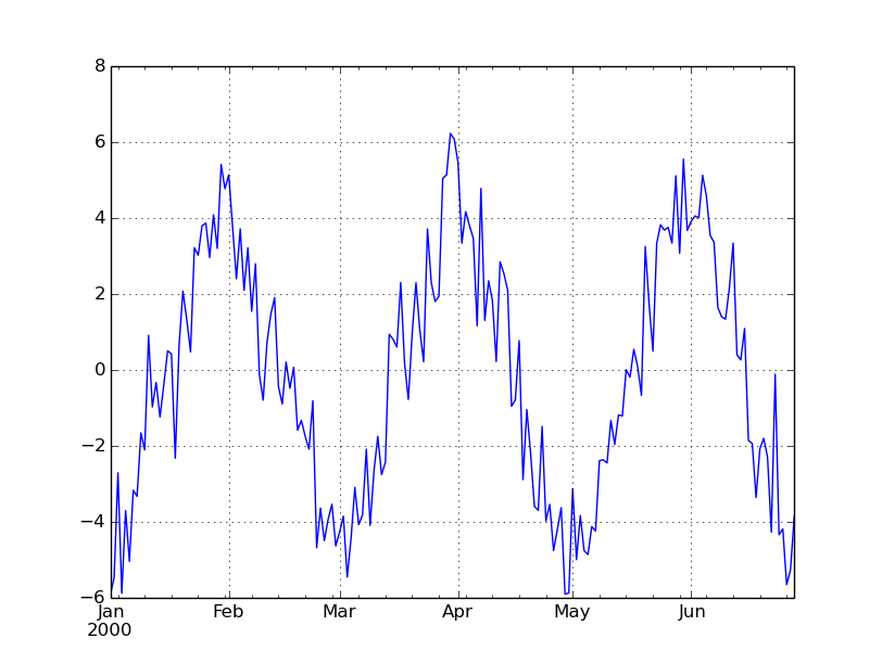
Using the python code here is the underlying process for one month trends over a 6 month period (Volscale=0.0 will add no noise, and so show us the underlying process):

ans=arbitrary_timeseries(generate_trendy_price(Nlength=180, Tlength=30, Xamplitude=10.0, Volscale=0.0)).plot()


Here is one random series with noise of 10% of the amplitude added on:

ans=arbitrary_timeseries(generate_trendy_price(Nlength=180, Tlength=30, Xamplitude=10.0, Volscale=0.10)).plot()


And here again another random price series with five times the noise:

ans=arbitrary_timeseries(generate_trendy_price(Nlength=180, Tlength=30, Xamplitude=10.0, Volscale=0.50)).plot()


Random correlated asset returns


Spreadsheet: There is a great resource here; others are available on the internet

My python code is here
It's for three assets but you should be able to adapt it easily enough.

Here is an example of the python code running. Notice the code generates returns, these are cumulated up to make an equity curve.

SRlist=[.5, 1.0, 0.0]
clist=[.9,.5,-0.5]

threeassetportfolio(plength=5000, SRlist=SRlist,    clist=clist).cumsum().plot()

We'll be using this kind of random price data in the final post of this series (why you should use robust out of sample portfolio optimisation techniques).

Random backtest returns (equity curve) with skew


Spreadsheet: There are a number of resources on the internet showing how skewed returns can be generated in excel including this one.

My python code


From my python code here is an equity curve with an expected Sharpe Ratio of +0.5 and no skew (gaussian returns):

cum_perc(arbitrary_timeseries(skew_returns_annualised(annualSR=0.5, want_skew=0.0, size=2500))).plot()


Now the same sharpe but with skew of +1 (typical of a relatively fast trend following system):

cum_perc(arbitrary_timeseries(skew_returns_annualised(annualSR=0.5, want_skew=1.0, size=2500))).plot()


Here is a backtest with Sharpe 1.0 and skew -3 (typical of a short gamma strategy such as relative value fixed income trading or option selling):

cum_perc(arbitrary_timeseries(skew_returns_annualised(annualSR=1.0, want_skew=-3.0, size=2500))).plot()

Ah the joys of compounding. But look out for the short, sharp, shocks of negative skew.

We'll use this python code again in the example at the end of this post (and in the next post on trading the equity curve).


Safe use of random data


What can we use random data for?


Some things that I have used random data for in the past include:

  • Looking at the correlation of trading rule returns
  • Seeing how sensitive optimal parameters are over different backtests
  • Understanding the likely holding period, and so trading costs, of different trading rules
  • Understanding how a trading rule will react to a given market event (eg 1987 stock market crash being repeated) or market environment (rising interest rates)
  • Checking that a trading rule behaves the way you expect - picks up on trends of a given length, handles corners cases and missing data, reduces positions at a given speed for a reversal of a given severity
  • Understanding how long it takes to get meaningful statistical information about asset returns and correlations
  • Understanding how to use different portfolio optimisation techniques; for example if using a Bayesian technique calibrating how much shrinkage to use (to be covered in the final post of this series)
  • Understanding the likely properties of strategy account curves (as in the example below)
  • Understanding the effects of modifying capital at risk in a drawdown (eg using Kelly scaling or 'trading the equity curve' as I'll talk about in the next post in this series)
[If you've read my book, "Systematic Trading", then you'll recognise many of the applications listed here]


What shouldn't we use random data for?


Random data cannot tell you how profitable a trading rule was in the past (or will be in the future... but then nothing can tell you that!). It can't tell you what portfolio weights to give to instruments or trading rule variations. For that you need real data, although you should be very careful - the usual rules about avoiding overfitting, and fitting on a pure out of sample basis apply.


Random data in a strategy design workflow


Bearing in mind the above I'd use a mixture of random and real data as follows when designing a trading strategy:

  • Using random data design a bunch of trading rule variations to capture the effects I want to exploit, eg market trends that last a month or so
  • Design and calibrate method for allocating asset weights with uncertainty, using random data (I'll cover this in the final post of this series)
  • Use the allocation method and real data to set the forecast weights (allocations to trading rule variations) and instrument weights; on a pure out of sample basis (eg expanding window).
  • Using random data decide on my capital scaling strategy - volatility target, use of Kelly scaling to reduce positions in a drawdown, trade the equity curve and so on (I'll give an example of this in the next post of this series).
Notice we only use real data once - the minimum possible.

Example: Properties of back tested equity curves


To finish this post let's look at a simple example. Suppose you want to know how likely it is that you'll see certain returns in a given live trading record; based on your backtest. You might be interested in:

  • The average return, volatility and skew.
  • The likely distribution of daily returns
  • The likely distribution of drawdown severity
To do this we're going to assume that:

  • We know roughly what sharpe ratio to expect (from a backtest or based on experience)
  • We know roughly what skew to expect (ditto)
  • We have a constant volatility target (this is arbitrary, let's make it 20%) which on average we achieve
  • We reduce our capital at risk when we make losses according to Kelly scaling (i.e. a 10% fall in account value means a 10% reduction in risk; in practice this means we deal in percentage returns)
Python code is here 

Let's go through the python code and see what it is doing (some lines are missed out for clarity). First we create 1,000 equity curves, with the default annualised volatility target of 20%. If your computer is slow, or you have no patience, feel free to reduce the number of random curves.

length_backtest_years=10
number_of_random_curves=1000

annualSR=0.5
want_skew=1.0

random_curves=[skew_returns_annualised(annualSR=annualSR, want_skew=want_skew, size=length_bdays)
               for NotUsed in range(number_of_random_curves)]


We can then plot these:

plot_random_curves(random_curves)
show()


Each of the light lines is a single equity curve. Note to make the effects clearer here I am adding up percentage returns, rather than applying compound interest properly. Alternatively I could graph the equity curves on a log scale to get the same picture.

All have an expected Sharpe Ratio of 0.5, but over 10 years their total return ranges from losing 'all' their capital (not in practice if we're using Kelly scaling), to making 3 times our initial capital (again in practice we'd make more).

The dark line shows the average of these curves. So on average we should expect to make our initial capital back (20% vol target, multiplied by Sharpe Ratio of 0.5, over 10 years). Notice that the cloud of equity curves around the average gives us an indication of how uncertain our actual performance over 10 years will be, even if we know for sure what the expected Sharpe Ratio is. This picture alone should convince you of how any individual backtest is just a random draw.

* Of course in the real world we don't know what the true Sharpe Ratio is. We just get one of the lighted coloured lines when we run a backtest on real financial data. From that we have to try and infer what the real Sharpe Ratio might be (assuming that the 'real' Sharpe doesn't change over time ... ). This is a very important point - never forget it.

Note that to do our analysis we can't just look at the statistics of the black line. It has the right mean return, but it is way too smooth! Instead we need to take statistics from each of the lighter lines, and then look at their distribution.


Magic moments


Mean annualised return


function_to_apply=np.mean
results=pddf_rand_data.apply(function_to_apply, axis=0)

## Annualise (not always needed, depends on the statistic)
results=[x*DAYS_IN_YEAR for x in results]

hist(results, 100)

As you'd expect the average return clusters around the expected value of 10% (With a Sharpe ratio of 0.5 and an annualised volatility target that is what you'd expect). But it's not unlikely that even over 10 years we'd see losses.


Volatility


function_to_apply=np.std
results=pddf_rand_data.apply(function_to_apply, axis=0)

## Annualise (not always needed, depends on the statistic)
results=[x*ROOT_DAYS_IN_YEAR for x in results]

hist(results, 100)


The realised annual standard deviation of returns is much more stable. Of course this isn't realistic. It doesn't account for the fact that a good trading system will reduce it's risk when opportunities are poor, and vice versa. It assumes we can always target volatility precisely, and that volatility doesn't unexpectedly change, or follow a different distribution to the skewed Gaussian we are assuming here.

But all those things apply equally to the mean - and that is still extremely unstable even in the simplified random world we're using here.


Skew


import scipy.stats as st
function_to_apply=st.skew
results=pddf_rand_data.apply(function_to_apply, axis=0)
 

hist(results, 100)


Skew is also relatively stable (in this simplified random world). I plotted this to confirm that the random process I'm using is reproducing the correct skew (in expectation).


Return distribution


function_to_apply=np.percentile
function_args=(100.0/DAYS_IN_YEAR,)
results=pddf_rand_data.apply(function_to_apply, axis=0, args=function_args)

hist(results, 100)
This graph answers the question "Over a 10 year period, how bad should I expect my typical worst 1 in 250 business day (once a year) loss to be?" (with the usual caveats). As an exercise for the reader you can try and reproduce similar results for different percentile points, and different return periods.


Drawdowns


Average drawdown


results=[x.avg_drawdown() for x in acccurves_rand_data]
hist(results, 100)


So most of the time an average drawdown of around 10 - 20% is expected. However there are some terrifying random equity curves where your average drawdown is over 50%.


Really bad drawdowns


results=[x.worst_drawdown() for x in acccurves_rand_data]
hist(results, 100)

So over 10 years you'll probably get a worst drawdown of around 40%. You might look at the backtest and think "I can live with that". However it's not impossible that you'll lose three quarters of your capital at times if you're unlucky. You really do have to be prepared to lose all your money.

Clearly I could continue and calculate all kinds of fancy statistics; however I'm hoping you get the idea and the code is hopefully clear enough.

What's next


As promised there will be two more posts in this series. In the next post I'll look at using random backtest returns to see if 'trading the equity curve' is a good idea.  Finally I'll explore why you should use robust  portfolio optimisation techniques rather than any alternative.

Monday, 2 November 2015

Typo in definition of carry rule for futures in "Systematic Trading" book

A thousand apologies but the definition of the carry rule for futures in Appendix B of my book "Systematic Trading" is incorrect.

This only applies to books printed before November 2019. Newer copies have this error corrected.

On page 287 of the print edition (Heading: The carry trading rule )

For 'Futures: If not trading nearest contract'

Instead of Current contract price minus nearer contract price

It should read Nearer contract price minus current contract price


For 'Futures: If trading nearest contract'

Instead of Next contract price minus current contract price

It should read Current contract price minus next contract price


The spreadsheet here was also wrong and is now corrected.

My python code was already correct; which is a relief as I use this rule in my own trading :-).

The figures and explanations of the rule in chapter seven are fine, as are the calculations for other asset classes in Appendix B.

I'd like to thank the reader (Raphael C) who pointed this error out to me.