I'm sometimes asked where I get my ideas for new trading strategies from. The boring truth is I rarely test new trading strategies, and I mostly steal ideas when I feel in the mood. Today for example I saw this tweet post on twitter X:
The original paper is here (requires subscription or academic institution membership)Think high market volatility leads to high returns? No. Periods with high market volatility are followed by high volatility, but not necessarily better returns. A volatility effect through time. Check out the graph below, based on the US equity market from 1927 to 2023. The… pic.twitter.com/23rrTwIf9O
— Pim van Vliet (@paradoxinvestor) October 2, 2023
Now I've written in the past about how volatility levels affect the profits of trading strategies, in particular momentum where there is a pretty striking effect (see my new book Advanced Futures Trading Strategies [AFTS] for more info), and I've also written about how the level of past vol affects future vol (and indeed, this incredible predictability of vol is a cornerstone of the inverse volatility sizing formula that lies at the heart of my trading strategies), but I don't think I've ever written about the level of volatility's effect on future price movements.
There is quite a simple story here which if you can see the paper is in figure 1: absolute returns are pretty flat across different vol regimes, and because vol is pretty autocorrelated from month to month, we'd expect return/vol to be higher if recent vol was lower. To put it another way, there is a link here with my previous post about CAPM; this story is sort of about the time series version of CAPM in which higher vol should be rewarded with higher returns (and hence Sharpe Ratios should not show any pattern conditional on relatively volatility levels), and the opposite happens in single stocks in an analogy to the fact that CAPM doesn't work in cross section for single stocks, in fact we should 'bet against beta' and buy low beta stocks.
But the paper is written for single stocks; a risky asset, and one with some idiosyncratic distributional features. Will the results hold for the wider universe of futures markets?
Data and definitions
I am not interested in reproducing the results in the paper since I'm more concerned with whether this is a profitable trading strategy sitting within my usual framework, so I will do things a bit differently.
I use my usual set of futures markets, after removing duplicates (eg micro and mini versions, or cross listings) it comes in at 211 instruments. Data goes back to 1970, and I use my standard vol estimate calculated in % terms, which I divide by an exponential moving average of the same with a 10 year vol halflife to get a relative vol measure. If this is 1, then the vol we're seeing is going to be typical of the level over the last couple of decades or so, if it's higher than 1 then the vol is higher, and so on. Again readers of AFTS will recognise this measure. The paper doesn't quite do this; it just looks at the level of vol versus the in sample historic distribution. This means we can't use that forecast as a trading signal.
For the y-axis of response, I will use the returns in the following month normalised by the volatility estimate (in price differences this time) at the beginning of the month for reasons I have discussed before. As I'm trading futures, this is also the Sharpe Ratio. The original paper uses a straight one month moving window of returns for vol estimation, and the pure ex-post Sharpe Ratio using the realised vol in the following month, so some small difference there. However because of the autocorrelation of vol, it shouldn't affect things too much; if anything my results probably should be a bit better because I'm dividing an unknown future estimate of mean by a known current estimate of standard deviation to get Sharpe Ratio, rather than having unknown mean/unknown sigma.
The original papers uses single stocks, I use a massive variety of futures allowing me to see if this effect persists at the stock index level and for other asset classes.
Some comparable graphs
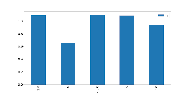
Let's start with producing the same kind of graphs as in the paper. So each month I look at the current level of vol versus it's historic average, and then rank it on an in sample basis (yes I know, but for the time being...), and then bucket the ranking into quintiles. I measure the risk adjusted return in the following month and take a median of those Sharpe Ratios; medians being somewhat more robust than mean.
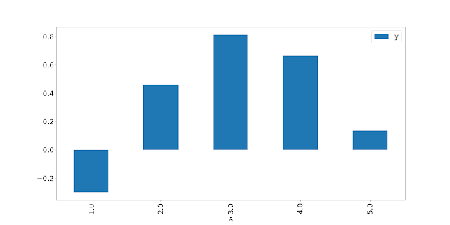
Here is the result for the S&P 500:
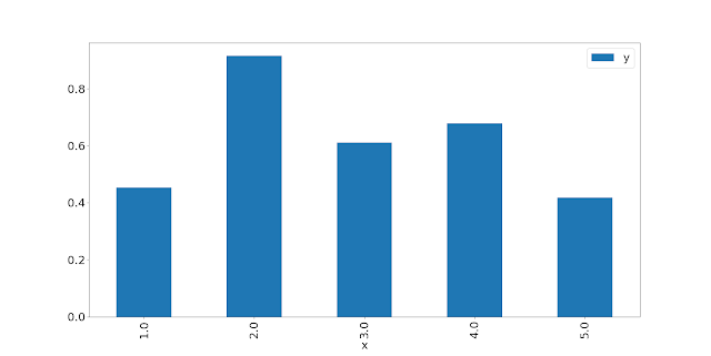
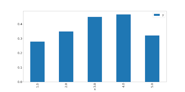
I use the same ordering; 1 on the left is the lowest quantile of vol, 5 on the right is the highest. That picture is not quite as compelling as the original paper; but ignoring the 2nd bar it has the right pattern: higher recent vol means lower risk adjusted returns in the following month. Nevertheless we are only using 492 data points compared to the thousands we can get with single stocks; plus I am suspicous of anyone that uses a single instrument to prove anything, so let's expand out to all equity futures (with months stacked, which will give a higher weight to instruments with more history):
That is .... not what we'd hoped for.
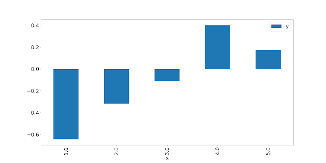
The name is Bond:
OK only two markets, but there is an apparent reverse effect here. You don't want to be long vol on average, but perhaps the worst time to be is when vol of vol is very low.
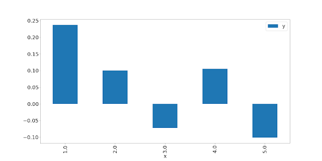
FX:
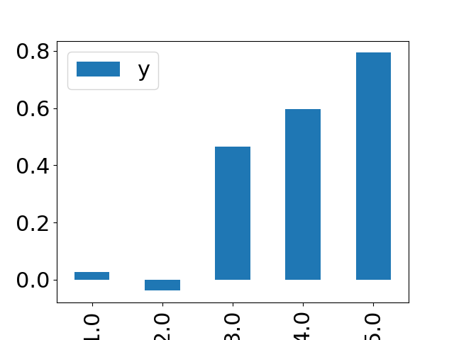
Just to give a point of comparison, here's the bucket plot if I replace the ratio of vol with the level of the 32/128 day momentum forecast level (something we know is very successful as a forecast at a portfolio level, although it is weak in say equities):
A trading rule
Although the results aren't what we expect, this could be profitable as a 'wrong way round' rule, which buys when vol is higher, and sells when vol is lower. This won't work for very high vol (since quintile 5 shows a worse return for quintiles 2,3 and 4, but then we would hit forecast capping up there anyway. That isn't much different to what happens with faster momentum rules anyway; if you plot response versus forecast level it's not as good for extreme forecasts (see AFTS for more).
In my first book, Systematic Trading, I said that implementing a rule as a wrong way rule after discovering it is a form of data mining so bear in mind that the backtest results here will effectively be overstated [in reality, you couldn't have implemented this rule until enough historical evidence that the effect was the 'wrong' way round existed; until that moment of statistically significant realisation we would eithier be trading the money losing 'right way round' rule, or a combination of the two, eithier of which is inferior to being all in on 'wrong way round' from the start of the backtest].
I'd add a couple of tweaks as well; firstly rather than quantile buckets which are too coarse and in sample; I will use the percentile of the ratio versus historic levels as the forecast (the same approach I use for the volatility overlay rule in AFTS) , and also chuck in my standard ewm(span=10) smooth to reduce noise on what should be a monthly holding forecast (this reduces turnover from 25 times a year to 10 times without affecting profitability).
Before continuing, it might be worth thinking about how this interacts with the volatility overlay on a trend following rule (which cuts exposure long or short when vol is high).
- If vol is low, we'd be SHORT from a vol rule
- ... and we'd have a stronger trend following signal
- if markets are trending up we'd be net flat
- If markets are trending down we'd have a strong sell
- If vol sits in the middle, we'd be FLAT from a vol rule
- .... and we've have an unadulterated trend signal
- If markets are trending up we'd be long
- If markets are trending down we'd be short
- If vol is high, we'd be LONG from a vol rule
- .... and have a weaker trend following signal
- If markets are trending up we'd be modestly long
- If markets are trending down we'd be flat
Other markets - which form the majority of futures instruments - will be less clear, so let's see how it goes.
Here's the code for the purely backward looking vol quantile calculation, and the actual trading rule:
def get_vol_quantile_points(self, instrument_code):
    self.log.debug("Calculating vol quantile for %s" % instrument_code)
    daily_vol = self.parent.rawdata.get_daily_percentage_volatility(instrument_code)
    ten_year_vol = daily_vol.rolling(2500, min_periods=10).mean()
    normalised_vol = daily_vol / ten_year_vol

    normalised_vol_q = quantile_of_points_in_data_series(normalised_vol)

    return normalised_vol_q
def quantile_of_points_in_data_series(data_series: pd.Series) -> pd.Series:
    ## With thanks to https://github.com/PurpleHazeIan for this implementation
    numpy_series = np.array(data_series)
    results = []

    for irow in range(len(data_series)):
        current_value = numpy_series[irow]
        count_less_than = (numpy_series < current_value)[:irow].sum()
        results.append(count_less_than / (irow + 1))

    results_series = pd.Series(results, index=data_series.index)
    return results_series
def vol_rule(vol_quantile_points: pd.Series, smooth: int = 10):
    # vol quantile points sits in space 0 to 1.0
    raw_forecast = (vol_quantile_points - 0.5) * 40  ## sits in space -20 to +20
    smoothed_forecast = raw_forecast.ewm(span=smooth).mean()
    return smoothed_forecast

