Equities, Bonds and maximising CAGR

Lots of things have changed in the last year. Many unthinkable things are now thinkable. A war in Europe. The UK coming 2nd in the Eurovision song contest rather than the usual dismal 'null points'. And of course, the correlation of stocks and bonds has recently gone more positive than it has been for over 20 years:

Rolling 12 month correlation of weekly returns for S&P 500 equity and US 10 year bond futures

I thought it would be 'fun' to see how the optimal stock/bond portfolio is affected by correlation and expected return assumptions.

In my second book, Smart Portfolios, I noted that a 100% equity portfolio made no sense under the Kelly criteria (AKA maximising CAGR), and that pretty much everyone should have some exposure to bonds regardless of their risk tolerance, even though they will have a lower expected arithmetic return due to their lower risk. For a while my own strategic risk weighting has been 10% in bonds, equating to cash weights of around 80/20.

I am currently reviewing my long only portfolio and it seems as good a time as any to check that 80/20 still makes sense.

Simple python code is liberally scattered throughout.

Assumptions and base case

I'm assuming a two asset, fully invested portfolio with two assets: a global stock, and a global bond (including both government and corporates). Both assets are Gaussian normal and have a linear relationship, so I can use an approximation for geometric return.

I assume that the standard deviation of the stocks is around 20% and the bonds around 10% (it's gone up recently, can't think why). Furthermore, I assume that my central case for the expected return in stocks is around 8%, and 5% in bonds. That corresponds to a simple SR (without risk free rate) of 0.4 and 0.5 respectively; eg a SR advantage for bonds versus the average SR of 0.05.

(Real return expectations are taken from AQR plus an assumed 3% inflation)

My utility function is to maximise real CAGR, which in itself implies I will be fully invested. Note that means I will be at 'full Kelly' - something that isn't usually advised. However we're determining allocations here, not leverage, so it's probably not as dangerous as you might think.

import numpy as np
import pandas as pd


def calculate_cagr(
    correlation, equity_weight, mean_eq, mean_bo, stdev_eq=0.2, stdev_bo=0.1
):
    bond_weight = 1 - equity_weight
    mean_return = (equity_weight * mean_eq) + (bond_weight * mean_bo)
    variance = (
        ((equity_weight**2) * (stdev_eq**2))
        + ((bond_weight**2) * (stdev_bo**2))
        + 2 * bond_weight * equity_weight * stdev_bo * stdev_eq * correlation
    )

    approx_cagr = mean_return - 0.5 * variance

    return approx_cagr

Effect of correlation varying with base case assumptions

I'm going to vary the correlation between stocks and bonds, between -0.8 and +0.8

list_of_weight_indices = list(np.arange(0, 1, 0.001))

def iterate_cagr(correlation, mean_eq, mean_bo):
    cagr_list = [
        calculate_cagr(
            correlation=correlation,
            equity_weight=equity_weight,
            mean_bo=mean_bo,
            mean_eq=mean_eq,
        )
        for equity_weight in list_of_weight_indices
    ]
    return cagr_list


corr_list = list(np.arange(-0.8, 0.8, 0.1))
corr_list = [round(x, 1) for x in corr_list]
## plot correlation varying
results = dict(
    [(correlation, iterate_cagr(correlation, 0.08, 0.05)) for correlation in corr_list]
)

results = pd.DataFrame(results)
results.columns = corr_list

results.index = list_of_weight_indices

results.plot()

So each line on this plot is a different correlation level. The x-axis is the cash weight on equities, and the y-axis is the geometric return / CAGR. You can see that as correlations get less negative and then positive, we get less diversification from bonds, and a higher weight to equities.

Let's look at the maximum CAGR in each case;

def weight_with_max_cagr(correlation, mean_eq, mean_bo):
    cagr_list = iterate_cagr(correlation, mean_eq, mean_bo)
    max_cagr = np.max(cagr_list)
    index_of_max = cagr_list.index(max_cagr)
    wt_of_max = list_of_weight_indices[index_of_max]

    return wt_of_max


results = pd.Series(
    [weight_with_max_cagr(correlation, 0.08, 0.05) for correlation in corr_list],
    index=corr_list,
)

On the x-axis is the correlation, and on the y-axis is the weight to equities which maximises the CAGR. Remember, these are cash weights. You can see that with zero correlations my original cash weight of 80% in equities is about right. But if correlations go above around 0.4 there is no point owning any bonds at all.

Effect of SR varying 

Now let's see what happens when we tweak the relative SR. I'm going to vary the relative simple Sharpe Ratio (return/standard deviation) between -0.5 and +0.5, keeping the average at 0.45 (positive numbers mean that equities are better). Note that the base case abve is equivalent to a differential of -0.05, in favour of bonds. To begin with, let's keep the correlation fixed at zero. 

def means_from_sr_diff(sr_diff, avg_sr=0.45, stdev_eq=0.2, stdev_bo=0.1):
    ## higher sr_diff is better for equities
    sr_eq = avg_sr + sr_diff
    sr_bo = avg_sr - sr_diff

    mean_eq = sr_eq * stdev_eq
    mean_bo = sr_bo * stdev_bo

    return mean_eq, mean_bo


def weight_with_max_cagr_given_sr_diff(correlation, sr_diff):
    mean_eq, mean_bo = means_from_sr_diff(sr_diff)
    return weight_with_max_cagr(correlation, mean_eq, mean_bo)


# fix corr at zero
sr_diff_list = list(np.arange(-0.5, 0.5, 0.01))
results = pd.Series(
    [weight_with_max_cagr_given_sr_diff(0, sr_diff) for sr_diff in sr_diff_list],
    index=sr_diff_list,
)

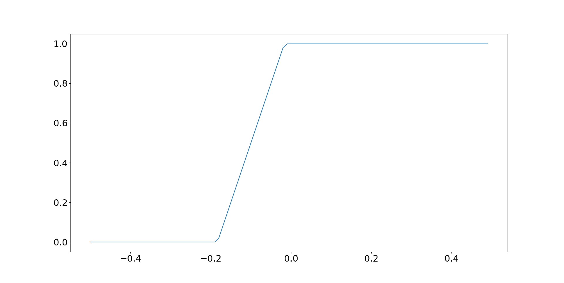
Just because CAGR isn't the mean return of standard mean variance optimisation, doesn't mean it won't suffer from the same problem of massive sensitivity to small differences in means (and Sharpe Ratios)! We wouldn't allocate *anything* to equities if the SR difference went below -0.2 (and which point the mean returns are 5% in equities and 6.5% in bonds), or anything to bonds if it's above -0.02 (8.7% in equities and 4.7% in bonds).  

Effect of SR and correlations varying 

sr_diff_list = list(np.arange(-0.25, 0.0501, 0.05))
sr_diff_list = [sr_diff.round(2) for sr_diff in sr_diff_list]
results = pd.DataFrame(
    dict(
        [
            (
                correlation,
                [
                    weight_with_max_cagr_given_sr_diff(correlation, sr_diff)
                    for sr_diff in sr_diff_list
                ],
            )
            for correlation in corr_list
        ]
    )
)

results.index = sr_diff_list
results.columns = corr_list

results = results.transpose()

results.plot()

Here again the x-axis is correlation, and the y-axis shows the weight to equities that maximises CAGR. 

Each of the lines on this plot is a different SR difference. The blue line has a SR advantage of 0.25 to bonds (label -0.25), and the light purple line (lillac?) is a small 0.05 SR advantage to equities. The brown line has no advantage to eithier asset class (misleadingly labelled -0.00 SR). The purple line is a -0.05SR advantage to bonds, which is equal to the base case I was using above - hence you can see the purple line matches the earlier plot of optimal weight versus correlation.

Notice that a SR advantage to bonds, SR difference = -0.1 (red line) results in 50% weights, irrespective of correlation. The lines above it, with a weaker advantage to bonds, put more in equities as correlations become more positive. The lillac line, SR difference 0.05, is 100% in equities, irrespective of correlations. The lines below the red line put less in equities as correlations become more positive.

Sensitivity

My usual base case is that expected SR differences between asset classes are zero, which implies I am somewhere on the brown line. Unless correlations are going to be somewhat negative, this implies 100% in equities. But the AQR base case figures for SR differences allow much more headroom for correlations. Even with correlations at the average 2022 level of around 0.30, one should still have a 10% cash weight in bonds.

How sensitive are my likely CAGR for the following 3 portfolios: 80% in equities, 90% and 100% in equities; over different assumptions of correlation and SR differential?

results = []
for correlation in [-0.4, 0, 0.4]:
    for sr_diff in [-0.25, 0, 0.25]:
        cagr80 = cagr_with_sr_diff(0.8, correlation, sr_diff)
        cagr90 = cagr_with_sr_diff(0.9, correlation, sr_diff)
        cagr100 = cagr_with_sr_diff(1, correlation, sr_diff)
        loss80 = cagr100 - cagr80
        loss90 = cagr100 - cagr90
        results.append(
            dict(
                correlation=correlation,
                sr_diff=sr_diff,
                cagr100=round(cagr100 * 100, 1),
                cagr90=round(cagr90 * 100, 1),
                cagr80=round(cagr80 * 100, 1),
                loss80=round(loss80 * 100, 2),
                loss90=round(loss90 * 100, 2),
            )
        )

print(pd.DataFrame(results))

  correlation  sr_diff  cagr100  cagr90  cagr80  loss80  loss90
0         -0.4    -0.25      2.0     2.7     3.4   -1.43   -0.75
1         -0.4     0.00      7.0     7.0     6.9    0.07    0.00
2         -0.4     0.25     12.0    11.2    10.4    1.57    0.75
3          0.0    -0.25      2.0     2.7     3.3   -1.30   -0.68
4          0.0     0.00      7.0     6.9     6.8    0.20    0.07
5          0.0     0.25     12.0    11.2    10.3    1.70    0.82
6          0.4    -0.25      2.0     2.6     3.2   -1.17   -0.60
7          0.4     0.00      7.0     6.9     6.7    0.33    0.15
8          0.4     0.25     12.0    11.1    10.2    1.83    0.90

For different scenarios of correlation and SR differential (positive better for equities remember), we can see the expected CAGR for portfolios with 100%, 90% and 80% in equities. 10.0 means a CAGR of 10% a year. The final two columns show the loss for an 80% vs 100%, and 90% vs 100% portfolio. Positive numbers mean the lower % of equities is worse, negative means they have outperformed all equities. Eg 1.00 means that the relevant portfolio has a 1% lower CAGR than 100% equities would.

Conclusion

100% in equities is never going to wash for me. Even if correlations have risen, and even with equal SR differentials, I'd be uncomfortable running that. But my current strategic cash weighting of 80% in equities also feels a little low given that correlations are elevated; even if I buy the AQR differential in favour of bonds.

On balance I've decided to increase my strategic cash allocation to ~87% in equities, which corresponds to a risk weighting of 93%.

ESG - Extremely Serious Goalpost moving: Rob goes green

Just a quick one:

I'm moving the goalposts on my example long only portfolio using UK listed ETFs (original blog post is here), done in the spirit of my second book Smart Portfolios: 

I've replaced all the ETFs in that portfolio with ESG funds

This is something I've wanted to do for a while, but the availability of ESG funds has really exploded recently and now the coverage is good enough that I think it's realistic to run an entire portfolio with just ESG.

The criteria is similar to before: low TER, reasonable AUM and ideally a distributing fund; although I've had to be a bit more flexible as the choice obviously still isn't as good. 

My ESG criteria was simple: I used the ESG criteria checkbox in justetf.com; I am not going to get into an argument about good versus bad ESG as I'm not an expert on that subject. My logic is that any ESG fund is probably better for the environment than an average non ESG fund, even if on balance there are going to be varying degrees of ESG fund. The portfolio reflects what an average investor can achieve without doing vast amounts of research, or investing directly in the underlying stocks (which again, will require significant research).

The only fund I excluded on ESG grounds was LGGG, which is very ESG-lite and only seems to exclude companies that actively murder people (one of it's largest holdings is Exxon!). Inevitably there are a few categories where I just couldn't find a suitable ESG fund. I also added a new bond category, bond issues by multilateral institutions, which matches the fund MDBU.

Rather pleasingly, and much to my surprise, the like for like matched simple average of TER across all the various ETF is virtually unchanged from before: 0.23%, just 1bp higher. This may just reflect fee pressure in the industry generally - I haven't updated the fees of the original portfolio for a few years and they have probably come down a bit, or cheaper funds may be available that weren't around originally.

I've created a new spreadsheet with the new tickers and portfolio in; the old spreadsheet link is still around but won't be updated. 

The plan is also to move my own investments into these funds, although it might take a few years as I don't want to incur a massive capital gains tax bill in the process.

Percentage or price differences when estimating standard deviation - that is the question

In a lot of my work, including my new book, I use two different ways of measuring standard deviation. The first method, which most people are familiar with, is to use some series of recent percentage returns. Given a series of prices p_t you might imagine the calculation would be something like this:

Sigma_% = f([p_t - p_t-1]/p_t-1, [p_t-1 - p_t-2]/pt-2, ....)

NOTE: I am not concerned with the form that function f takes in this post, but for the sake of argument let's see it's a simple moving average standard deviation. So we would take the last N of these terms, subtract the rolling mean from them, square them, take the average, and then take the square root.

For futures trading we have two options for p_t: the 'current' price of the contract, and the back adjusted price. These will only be the same in the days since the last roll. In fact, because the back adjusted price can go to zero or become negative, I strongly advocate using the 'current' price as the denominator in the above equation, and the changein back adjusted price as the numerator. If we used the change in current price, we'd see a pop upwards in volatility every time there was a futures roll. So if p*_t is the current price of a contract, then:

Sigma_% = f([p_t - p_t-1]/p*_t-1, [p_t-1 - p_t-2]/p*t-2, ....)

The alternative method, is to use some series of price differences:

Sigma_d = f([p_t - p_t-1], [p_t-1 - p_t-2], ....)

Here these are all 

If I wanted to convert this standard deviation into terms comparable with the % standard deviation, then I would divide this by the current price (*not* the backadjusted price):

Sigma_d% = Sigma_d / p*_t

Now, clearly these are not going to give exactly the same answer, except in the tedious case where there has been no volatility (and perhaps a few, other, odd corner cases). This is illustrated nicely by the following little figure-ette (figure-ine? figure-let? figure-ling?):

import pandas as pd
perc =(px.diff()/pxc.shift(1)).rolling(30, min_periods=3).std()
diff = (px.diff()).rolling(30, min_periods=3).std().ffill()/pxc.ffill()
both = pd.concat([perc,diff], axis=1)
both.columns = ['%', 'diff']

The two series are tracking pretty closely, except in the extreme vol of late 2008, and even they aren't that different. 

Here is another one:

That's WTi crude oil during COVID; and there is quite a big difference there. Incidentally, the difference could have been far worse. I was trading the December 2020 contract at the time... the front contract in this period (May 2020) went below zero for several days.

Now most people are more familiar with % standard deviations, which is why I have used it so much, but what you may not realise is that the price difference standard deviation is far more important.

How come? Well consider the basic position sizing equation that I have used throughout my work:

N = Capital × τ ÷ (Multiplier × Price × FX rate × σ_% )

(This is the version in my latest book, but very similar versions appear in my first and third books). Ignoring most things we get:

N = X ÷ (Price × σ_%)

So the number of contracts held is proportional to one divided by the price multiplied by the percentage standard deviation estimate. The price shown is, if you've been paying attention, the current price not the back adjusted one. But remember:

Sigma_d% = Sigma_d / p*_t

Hence the position is actually proportional to the standard deviation in price difference terms. We can eithier estimate this directly, or as the equation suggests recover it from the standard deviation in percentage terms, which we then multiply by the current futures price.

As the graphs above suggest, in the majority of cases it won't make much difference which of these methods you choose. But for the corner case of prices close to zero, it will be more robust to use price differences. In conclusion: I recommend using price differences to estimate the standard deviation.

Finally, there are also times when it still makes sense to use % returns. For example, when estimating risk it's more natural to do this using percentages (I do this when getting a covariance matrix for my exogenous risk overlay and dynamic optimisation). When percentage standard deviation is required I usually divide my price difference estimate by the absolute value of the current futures price. That will handle prices close to zero and negative prices, but it will result in temporarily very high % standard deviations. This is mostly unavoidable, but at least the problem is confined to a small part of the strategy, and the most likely outcome is that we won't take positions in these markets (probably not a bad thing!).

Footnote: Shout out to the diff(log price) people. How did those negative prices work out for you guys?